Meaning: Octorokus from [octorok] in Hylian; infletus from [inflate] in Latin.
Translation: inflating octorok; all varieties use an inflatable air sac derived from the swim bladder to float and scan the horizon.
Varieties
Octorokus infletus hydros [aquatic morphotype]
Octorokus infletus petram [mountain morphotype]
Octorokus infletus silva [forest morphotype]
Octorokus infletus arctus [snow morphotype]
Octorokus infletus imitor [deceptive morphotype]
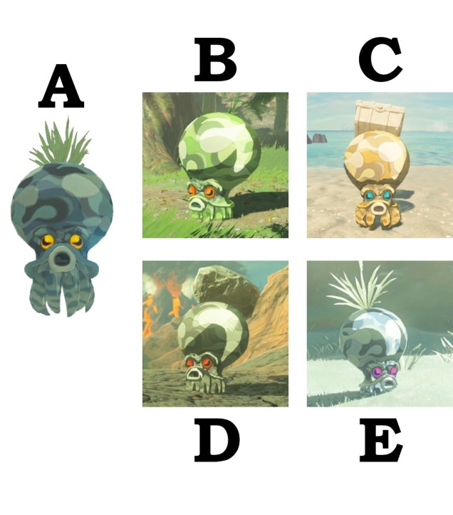
The various morphotypes of inflating octoroks. A: The water octorok, considered the morphotype closest to the ancestral physiology of the species. B: The forest octorok, with grass camouflage. C: The deceptive octorok, which has replaced its tufted vegetation with a glittering chest as bait. D: The mountainous octorok, with rock camouflage. E: The snow octorok, with tundra grass camouflage.
Common name
Variable octorok
Taxonomic status
Kingdom Animalia; Phylum Mollusca; Class Cephalapoda; Order Octopoda; Family Octopididae; GenusOctorokus; Speciesinfletus
Conservation status
Least Concern
Distribution
The species is found throughout all major habitat regions of Hyrule, with localised morphotypes found within specific habitats. The only major region where the variable octorok is not found is within the Gerudo Desert, suggesting some remnant dependency of standing water.
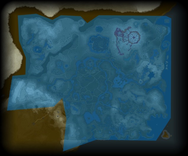
The region of Hyrule, with the distribution of octoroks in blue. The only major region where they are not found is the Gerudo Desert in the bottom left.
Habitat
Habitat choice depends on the physiology of the morphotype; so long as the environment allows the octorok to blend in, it is highly likely there are many around (i.e. unseen).
Behaviour and ecology
The variable octorok is arguably one of the most diverse species within modern Hyrule, exhibiting a large number of different morphotypic forms and occurring in almost all major habitat zones. Historical data suggests that the water octorok (Octorokus infletus hydros) is the most ancestral morphotype, with ancient literature frequently referring to them as sea-bearing or river-traversing organisms. Estimates from the literature suggests that their adaptation to land-based living is a recent evolutionary step which facilitated rapid morphological radiation of the lineage.
Several physiological characteristics unite the variable morphological forms of the octorok into a single identifiable species. Other than the typical body structure of an octopod (eight legs, largely soft body with an elongated mantle region), the primary diagnostic trait of the octorok is the presence of a large ‘balloon’ with the top of the mantle. This appears to be derived from the swim bladder of the ancestral octorok, which has shifted to the cranial region. The octorok can inflate this balloon using air pumped through the gills, filling it and lifting the octorok into the air. All morphotypes use this to scan the surrounding region to identify prey items, including attacking people if aggravated.
A water morphotype octorok with balloon inflated.
Diets of the octorok vary depending on the morphotype and based on the ecological habitat; adaptations to different ecological niches is facilitated by a diverse and generalist diet.
Demography
Although limited information is available on the amount of gene flow and population connectivity between different morphotypes, by sheer numbers alone it would appear the variable octorok is highly abundant. Some records of interactions between morphotypes (such as at the water’s edge within forested areas) implies that the different types are not reproductively isolated and can form hybrids: how this impacts resultant hybrid morphotypes and development is unknown. However, given the propensity of morphotypes to be largely limited to their adaptive habitats, it would seem reasonable to assume that some level of population structure is present across types.
Adaptive traits
The variable octorok appears remarkably diverse in physiology, although the recent nature of their divergence and the observed interactions between morphological types suggests that they are not reproductively isolated. Whether these are the result of phenotypic plasticity, and environmental pressures are responsible for associated physiological changes to different environments, or genetically coded at early stages of development is unknown due to the cryptic nature of octorok spawning.
All octoroks employ strong behavioural and physiological traits for camouflage and ambush predation. Vegetation is usually placed on the top of the cranium of all morphotypes, with the exact species of plant used dependent on the environment (e.g. forest morphotypes will use grasses or ferns, whilst mountain morphotypes will use rocky boulders). The octorok will then dig beneath the surface until just the vegetation is showing, effectively blending in with the environment and only occasionally choosing to surface by using the balloon. Whether this behaviour is passed down genetically or taught from parents is unclear.
Management actions
Few management actions are recommended for this highly abundant species. However, further research is needed to better understand the highly variable nature and the process of evolution underpinning their diverse morphology. Whether morphotypes are genetically hardwired by inheritance of determinant genes, or whether alterations in gene expression caused by the environmental context of octoroks (i.e. phenotypic plasticity) provides an intriguing avenue of insight into the evolution of Hylian fauna.
Nevertheless, the transition from the marine environment onto the terrestrial landscape appears to be a significant stepping stone in the radiation of morphological structures within the species. How this has been facilitated by the genetic architecture of the octorok is a mystery.
Meaning: Cinis: from [ash] in Latin; descendens from [descends] in Latin.
Translation: descending from the ash; describes hunting behaviour in ash mountains of Vvardenfell.
Common name
Cliff racer
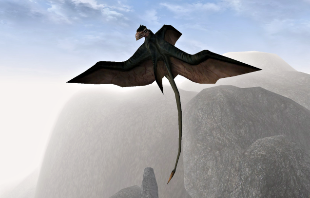
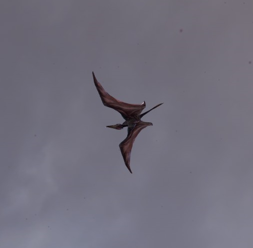
A cliff racer hovering above a precipice on Vvardenfell.
Taxonomic status
Kingdom Animalia; Phylum Chordata; Class Aves; Subclass Archaeornithes; Family Vvardidae; GenusCinis; Speciesdescendens
Conservation status
Least Concern [circa 3E 427]
Threatened [circa 4E 433]
Distribution
Once widespread throughout the north eastern region of Tamriel, occupying regions from the island of Vvardenfell to mainland Morrowind and Solstheim. Despite their name, the cliff racer is found across nearly all geographic regions of Vvardenfell, although the species is found in greatest densities in the rocky interior region of Stonefalls.
Following a purge of the species as part of pest control management, the cliff racer was effectively exterminated from parts of its range, including local extinction on the island of Solstheim. Since the cull the cliff racer is much less abundant throughout its range although still distributed throughout much of Vvardenfell and mainland Morrowind.
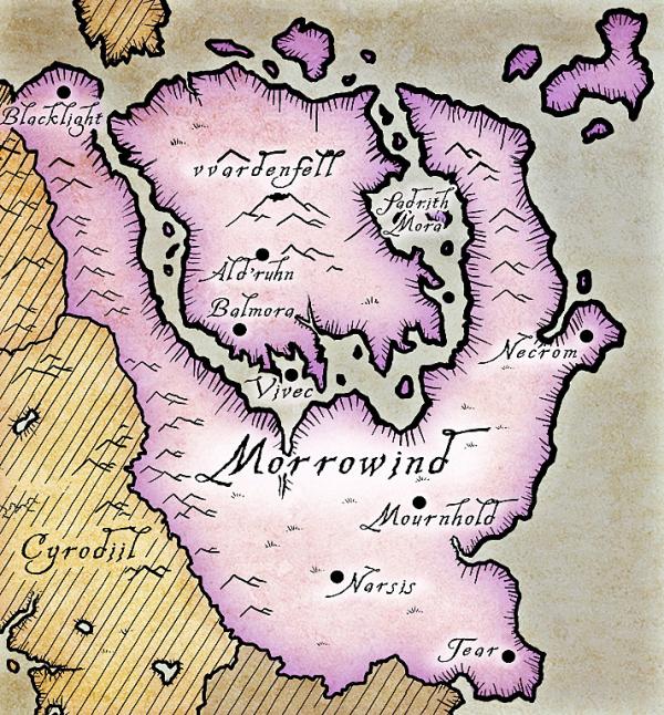
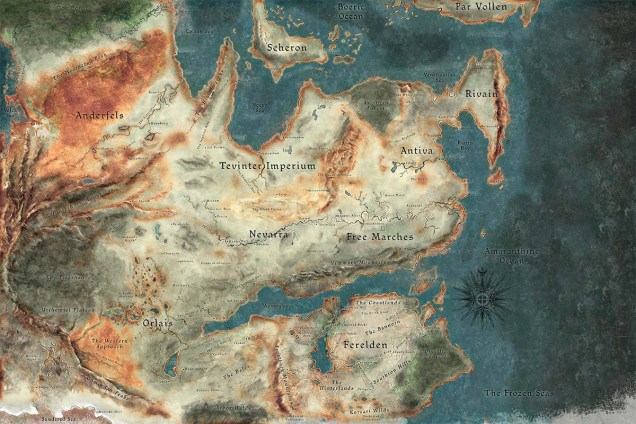
The province of Morrowind, which largely contains the distribution of the cliff racer. The island of Solstheim is found to the northwest of the map (the lower half of the island can be seen in brown).
Habitat
Although, much as the name suggests, the cliff racer prefers rocky outcroppings and mountainous regions in which it can build its nest, the species is frequently seen in lowland swamp and plains regions of Morrowind.
Behaviour and ecology
The cliff racer is a highly aggressive ambush predator, using height and range to descend on unsuspecting victims and lashing at them with its long, sharp tail. Although preferring to predate on small rodents and insects (such as kwama), cliff racers have been known to attack much larger beasts such as agouti and guar if provoked or desperate. The highly territorial nature of cliff racer means that they often attack travellers, even if they pose no immediate threat or have done nothing to provoke the animal.
A cliff racer descends upon its prey.
Despite the territoriality of cliff racers, large flocks of them can often be found in the higher altitude regions of Vvardenfell, perhaps facilitated by an abundance of food (reducing competition) or communal breeding grounds. Attempts by researchers to study these aggregations have been limited due to constant attacks and damage to equipment by the flock.
Following the control measures implemented, the population size of these populations of cliff racers declined severely; however, given the survival of the majority of the population it does not appear this bottleneck has severely impacted the longevity of the species. The extirpation of the Solstheim population of cliff racers likely removed a unique ESU from the species, given the relative isolation of the island. Whether the island will be recolonised in time by Vvardenfell cliff racers is unknown, although the presence of any cliff racers back onto Solstheim would likely be met with strong opposition from the local peoples.
Adaptive traits
The broad wings, dorsal sail and long tail allow the cliff racer to travel large distances in the air, serving them well in hunting behaviour. The drawback of this is that, if hunting during the middle hours of the day, the cliff racer leaves an imposing shadow on the ground and silhouette in the sky, often alerting aware prey to their presence. That said, the speed of descent and disorienting cry of the animal often startles prey long enough for the cliff racer to attack.
The plumes of the cliff racer are a well-sought-after commodity by local peoples, used in the creation of garments and household items. Whether these plumes serve any adaptive purpose (such as sexual selection through mate signalling) is unknown, given the difficulties with studying wild cliff racer behaviour.
Management actions
Although suffering from a strong population bottleneck after the purge, the cliff racer is still relatively abundant across much of its range and maintains somewhat stable size. Management and population control of the cliff racer is necessary across the full distribution of the species to prevent strong recovery and maintain public safety and ecosystem balance. Breeding or rescuing cliff racers is strictly forbidden and the species has been widely declared as ‘native pest’, despite the somewhat oxymoron nature of the phrase.
Nugs are non-confrontational omnivorous species, preferring to hide and delve in the dark underground systems below the world of Thedas. Thus, nugs will typically avoid contact with people or predators by hiding in various crevices, using their pale skin to blend in with the surrounding rock faces. Reports of nugs in the wild demonstrate that nugs are remarkably inefficient at predator avoidance, despite their physiology; however, nug populations do not appear to suffer dramatically with predator presence, suggesting that either predators are too few to significantly impact population size or that alternative behaviours might allow them to rapidly bounce back from natural declines.
Given the lack of consistent light within their habitat, nugs are effectively blind, retaining only limited eyesight required for moving around above the surface. Nugs feed on a large variety of food sources, preferring insects but resorting to mineral deposits if available food resources are depleted. Their generalist diet may be one physiological trait that has allowed the nug to become some widespread and abundant historically.
Demography
Although the nug is a widespread and abundant species, they are heavily reliant on the connections of the Deep Roads to maintain connectivity and gene flow. With the gradual declination of Dwarven abundance and the loss of entire regions of the underground civilisation, it is likely that many areas of the nug distribution have become isolated and suffering from varying levels of inbreeding depression. Given the lack of access to these populations, whether some have collapsed since their isolation is unknown and potentially isolated populations may have even speciated if local environments have changed significantly.
Adaptive traits
Nugs are highly adapted to low-light, subterranean conditions, and show many phenotypic traits related to this kind of environment. The reduction of eyesight capability is considered a regression of unusable traits in underground habitats; instead, nugs show a highly developed and specialised nasal system. The high sensitivity of the nasal cavity makes them successful forages in the deep caverns of the underworld, and the elongated maw of the nug allows them to dig into buried food sources with ease. One of the more noticeable (and often disconcerting) traits of the nug is their human-like hands; the development of individual digits similar to fingers allows the nug to grip and manipulate rocky surfaces with surprising ease.
Management actions
Re-establishment of habitat corridors through the clearing and revival of the Deep Roads is critical for both reconnecting isolated populations of nugs and restoring natural gene flow, but also allowing access to remote populations for further studies. A combination of active removal of resident Darkspawn and population genetics analysis to accurately assess the conservation status of the species. That said, given the commercial value of the nug as a food source for many societies, establishing consistent sustainable farming practices may serve to both boost the nug populations and also provide an industry for many people.
This is the fourth (and final) part of the miniseries on the genetics and process of speciation. To start from Part One, click here.
In last week’s post, we looked at how we can use genetic tools to understand and study the process of speciation, and particularly the transition from populations to species along the speciation continuum. Following on from that, the question of “how many species do I have?” can be further examined using genetic data. Sometimes, it’s entirely necessary to look at this question using genetics (and genomics).
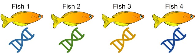
An example of cryptic species. All four fish in this figure are morphologically identical to one another, but they differ in their underlying genetic variation (indicated by the different colours of DNA). Thus, from looking at these fish alone we would not perceive any differences, but their genetic make-up might suggest that there are more than one species…The level of genetic differentiation between the fish in the above example. The phylogenies on the left and top of the figure demonstrate the evolutionary relationships of these four fish. The matrix shows a heatmap of the level of differences between different pairwise comparisons of all four fish: red squares indicate zero genetic differences (such as when comparing a fish to itself; the middle diagonal) whilst yellow squares indicate increasingly higher levels of genetic differentiation (with bright yellow = all differences). By comparing the different fish together, we can see that Fish 1 and 2, and Fish 3 and 4, are relatively genetically similar to one another (red-deep orange). However, other comparisons show high level of genetic differences (e.g. 1 vs 3 and 1 vs 4). Based on this information, we might suggest that Fish 1 and 2 belong to one cryptic species (A) and Fish 3 and 4 belong to a second cryptic species (B).
Genetic tools to study species: the ‘Barcode of Life’
A classically employed method that uses DNA to detect and determine species is referred to as the ‘Barcode of Life’. This uses a very specific fragment of DNA from the mitochondria of the cell: the cytochrome c oxidase I gene, CO1. This gene is made of 648 base pairs and is found pretty well universally: this and the fact that CO1 evolves very slowly make it an ideal candidate for easily testing the identity of new species. Additionally, mitochondrial DNA tends to be a bit more resilient than its nuclear counterpart; thus, small or degraded tissue samples can still be sequenced for CO1, making it amenable to wildlife forensics cases. Generally, two sequences will be considered as belonging to different species if they are certain percentage different from one another.
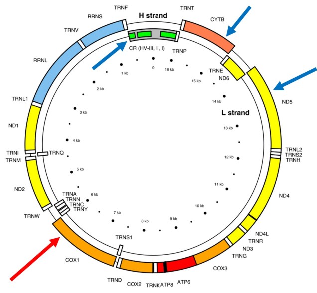
The full (annotated) mitochondrial genome of humans, with the different genes within it labelled. The CO1 gene is labelled with the red arrow (sometimes also referred to as COX1) whilst blue arrows point to other genes often used in phylogenetic or taxonomic studies, depending on the group or species in question.
Despite the apparent benefits of CO1, there are of course a few drawbacks. Most of these revolve around the mitochondrial genome itself. Because mitochondria are passed on from mother to offspring (and not at all from the father), it reflects the genetic history of only one sex of the species. Secondly, the actual cut-off for species using CO1 barcoding is highly contentious and possibly not as universal as previously suggested. Levels of sequence divergence of CO1 between species that have been previously determined to be separate (through other means) have varied from anywhere between 2% to 12%. The actual translation of CO1 sequence divergence and species identity is not all that clear.
Gene tree – species tree incongruences
One particularly confounding aspect of defining species based on a single gene, and with using phylogenetic-based methods, is that the history of that gene might not actually be reflective of the history of the species. This can be a little confusing to think about but essentially leads to what we call “gene tree – species tree incongruence”. Different evolutionary events cause different effects on the underlying genetic diversity of a species (or group of species): while these may be predictable from the genetic sequence, different parts of the genome might not be as equally affected by the same exact process.
A classic example of this is hybridisation. If we have two initial species, which then hybridise with one another, we expect our resultant hybrids to be approximately made of 50% Species A DNA and 50% Species B DNA (if this is the first generation of hybrids formed; it gets a little more complicated further down the track). This means that, within the DNA sequence of the hybrid, 50% of it will reflect the history of Species A and the other 50% will reflect the history of Species B, which could differ dramatically. If we randomly sample a single gene in the hybrid, we will have no idea if that gene belongs to the genealogy of Species A or Species B, and thus we might make incorrect inferences about the history of the hybrid species.
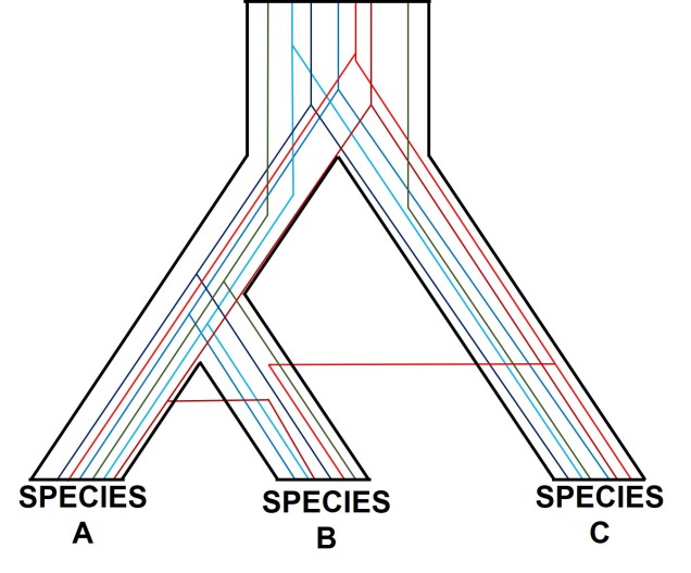
A diagram of gene tree – species tree incongruence. Each individual coloured line represents a single gene as we trace it back through time; these are mostly bound within the limits of species divergences (the black borders). For many genes (such as the blue ones), the genes resemble the pattern of species divergences very well, albeit with some minor differences in how long ago the splits happened (at the top of the branches). However, the red genes contrast with this pattern, with clear movement across species (from A and C into B): this represents genes that have been transferred by hybridisation. The green line represents a gene affected by what we call incomplete lineage sorting; that is, we cannot trace it back far enough to determine exactly how/when it initially diverged and so there are still two separate green lines at the very top of the figure. You can think of each line as a separate phylogenetic tree, with the overarching species tree as the average pattern of all of the genes.
There are a number of other processes that could similarly alter our interpretations of evolutionary history based on analysing the genetic make-up of the species. The best way to handle this is simply to sample more genes: this way, the effect of variation of evolutionary history in individual genes is likely to be overpowered by the average over the entire gene pool. We interpret this as a set of individual gene trees contained within a species tree: although one gene might vary from another, the overall picture is clearer when considering all genes together.
Species delimitation
In earlier posts on The G-CAT, I’ve discussed the biogeographical patterns unveiled by my Honours research. Another key component of that paper involved using statistical modelling to determine whether cryptic species were present within the pygmy perches. I didn’t exactly elaborate on that in that section (mostly for simplicity), but this type of analysis is referred to as ‘species delimitation’. To try and simplify complicated analyses, species delimitation methods evaluate possible numbers and combinations of species within a particular dataset and provides a statistical value for which configuration of species is most supported. One program that employs species delimitation is Bayesian Phylogenetics and Phylogeography(BPP): to do this, it uses a plethora of information from the genetics of the individuals within the dataset. These include how long ago the different populations/species separated; which populations/species are most related to one another; and a pre-set minimum number of species (BPP will try to combine these in estimations, but not split them due to computational restraints). This all sounds very complex (and to a degree it is), but this allows the program to give you a statistical value for what is a species and what isn’t based on the genetics and statistical modelling.
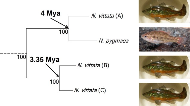
The cryptic species of pygmy perches identified within my research paper. This represents part of the main phylogenetic tree result, with the estimates of divergence times from other analyses included. The pictures indicate the physiology of the different ‘species’: Nannoperca pygmaea is morphologically different to the other species of Nannoperca vittata. Species delimitation analysis suggested all four of these were genetically independent species; at the very least, it is clear that there must be at least 2 species of Nannoperca vittata since A is more related to N. pygmaea than to other N. vittata species. Photo credits: N. vittata = Chris Lamin; N. pygmaea = David Morgan.
The end result of a BPP run is usually reported as a species tree (e.g. a phylogenetic tree describing species relationships) and statistical support for the delimitation of species (0-1 for each species). Because of the way the statistical component of BPP works, it has been found to give extremely high support for species identities. This has been criticised as BPP can, at time, provide high statistical support for genetically isolated lineages (i.e. divergent populations) which are not actually species.
Improving species identities with integrative taxonomy
Due to this particular drawback, and the often complex nature of species identity, using solely genetic information such as species delimitation to define species is extremely rare. Instead, we use a combination of different analytical techniques which can include genetic-based evaluations to more robustly assign and describe species. In my own paper example, we suggested that up to three ‘species’ of N. vittata that were determined as cryptic species by BPP could potentially exist pending on further analyses. We did not describe or name any of the species, as this would require a deeper delve into the exact nature and identity of these species.
As genetic data and analytical techniques improve into the future, it seems likely that our ability to detect and determine species boundaries will also improve. However, the additional supported provided by alternative aspects such as ecology, behaviour and morphology will undoubtedly be useful in the progress of taxonomy.
Given the strong influence of genetic identity on the process and outcomes of the speciation process, it seems a natural connection to use genetic information to study speciation and species identities. There is a plethora of genetics-based tools we can use to investigate how speciation occurs (both the evolutionary processes and the external influences that drive it). One clear way to test whether two populations of a particular species are actually two different species is to investigate genes related to reproductive isolation: if the genetic differences demonstrate reproductive incompatibilities across the two populations, then there is strong evidence that they are separate species (at least under the Biological Species Concept; see Part One for why!). But this type of analysis requires several tools: 1) knowledge of the specific genes related to reproduction (e.g. formation of sperm and eggs, genital morphology, etc.), 2) the complete and annotated genome of the species (to be able to find and analyse the right genes properly) and 3) a good amount of data for the populations in question. As you can imagine, for people working on non-model species (i.e. ones that haven’t had the same history and detail of research as, say, humans and mice), this can be problematic. So, instead, we can use other genetic information to investigate and suggest patterns and processes related to the formation of new species.
Is reproductive isolation naturally selected for or just a consequence?
A fundamental aspect of studies of speciation is a “chicken or the egg”-type paradigm: does natural selection directly select for rapid reproductive isolation, preventing interbreeding; or as a secondary consequence of general adaptive differences, over a long history of evolution? This might be a confusing distinction, so we’ll dive into it a little more.
Of the two proposed models of speciation, the by-product of natural selection (the second model) has been the more favoured. Simply put, this expands on Darwin’s theory of evolution that describes two populations of a single species evolving independently of one another. As these become more and more different, both in physical (‘phenotype’) and genetic (‘genotype’) characteristics, there comes a turning point where they are so different that an individual from one population could not reasonably breed with an individual from the other to form a fertile offspring. This could be due to genetic incompatibilities (such as different chromosome numbers), physiological differences (such as changes in genital morphology), or behavioural conflicts (such as solitary vs. group living).
Certainly, this process makes sense, although it is debatable how fast reproductive isolation would occur in a given species (or whether it is predictable just based on the level of differentiation between two populations). Another model suggests that reproductive isolation actually might arise very quickly if natural selection favours maintaining particular combinations of traits together. This can happen if hybrids between two populations are not particularly well adapted (fit), causing natural selection to favour populations to breed within each group rather than across groups (leading to reproductive isolation). Typically, this is referred to as ‘reinforcement’ and predominantly involves isolating mechanisms that prevent individuals across populations from breeding in the first place (since this would be wasted energy and resources producing unfit offspring). The main difference between these two models is the sequence of events: do populations ecologically diverge, and because of that then become reproductively isolated, or do populations selectively breed (enforcing reproductive isolation) and thus then evolve independently?
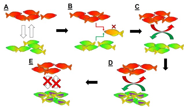
An example of reinforcement leading to speciation. A) We start with two populations of a single species (a red fish population and a green fish population), which can interbreed (the arrows). B) Because these two groups can breed, hybrids of the two populations can be formed. However, due to the poor combination of red and green fish genes within a hybrid, they are not overly fit (the red cross). C) Since natural selection doesn’t favour forming hybrids, populations then adapt to selectively breed only with similar fish, reducing the amount of interbreeding that occurs. D) With the two populations effectively isolated from one another, different adaptations specific to each population (spines in red fish, purple stripes in green fish) can evolve, causing them to further differentiate. E) At some point in the differentiation process, hybrids move from being just selectively unfit (as in B)) to entirely impossible, thus making the two populations formal species. In this example, evolution has directly selected against hybrids first, thus then allowing ecological differences to occur (as opposed to the other way around).
Reproductive isolation through DMIs
The reproductive incompatibility of two populations (thus making them species) is often intrinsically linked to the genetic make-up of those two species. Some conflicts in the genetics of Population 1 and Population 2 may mean that a hybrid having half Population 1 genes and half Population 2 genes will have serious fitness problems (such as sterility or developmental problems). Dramatic genetic differences, particularly a difference in the number of chromosomes between the two sources, is a significant component of reproductive isolation and is usually to blame for sterile hybrids such as ligers, zorse and mules.
However, subtler genetic differences can also have a strong effect: for example, the unique combination of Population 1 and Population 2 genes within a hybrid might interact with one another negatively and cause serious detrimental effects. These are referred to as “Dobzhansky-Müller Incompatibilities” (DMIs) and are expected to accumulate as the two populations become more genetically differentiated from one another. This can be a little complicated to imagine (and is based upon mathematical models), but the basis of the concept is that some combinations of gene variants have never, over evolutionary history, been tested together as the two populations diverge. Hybridisation of these two populations suddenly makes brand new combinations of genes, some of which may be have profound physiological impacts (including on reproduction).
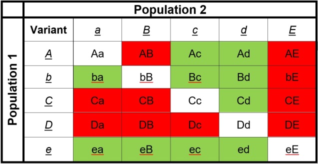
An example of how Dobzhansky-Müller Incompatibilities arise, adapted from Coyne & Orr (2004). We start with an initial population (center top), which splits into two separate populations. In this example, we’ll look at how 5 genes (each letter = one gene) change over time in the separate populations, with the original allele of the gene (lowercase) occasionally mutating into a new allele (upper case). These mutations happen at random times and in random genes in each population (the red letters), such that the two become very different over time. After a while, these two populations might form hybrids; however, given the number of changes in each population, this hybrid might have some combinations of alleles that are ‘untested’ in their evolutionary history (see below). These untested combinations may cause the hybrid to be infertile or unviable, making the two populations isolated species.The list of ‘untested’ genetic combinations from the above example. This table shows the different combinations of each gene that could be made in a hybrid if these two populations interbred. The red cells indicate combinations that have never been ‘tested’ together; that is, at no point in the evolutionary history of these two populations were those two particular alleles together in the same individual. Green cells indicate ones that were together at some point, and thus are expected to be viable combinations (since the resultant populations are obviously alive and breeding).
How can we look at speciation in action?
We can study the process of speciation in the natural world without focussing on the ‘reproductive isolation’ element of species identity as well. For many species, we are unlikely to have the detail (such as an annotated genome and known functions of genes related to reproduction) required to study speciation at this level in any case. Instead, we might choose to focus on the different factors that are currently influencing the process of speciation, such as how the environmental, demographic or adaptive contexts of populations plays a role in the formation of new species. Many of these questions fall within the domain of phylogeography; particularly, how the historical environment has shaped the diversity of populations and species today.
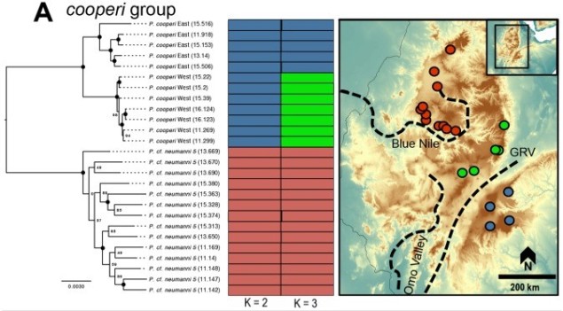
An example of the interplay between speciation and phylogeography, taken from Reyes-Velasco et al. (2018). They investigated the phylogeographic history of several different groups of species within the frog genus Ptychadena; in this figure, we can see how the different species (indicated by the colours and tree on the left) relate to the geography of their habitat (right).
A variety of different analytical techniques can be used to build a picture of the speciation process for closely related or incipient species. A good starting point for any speciation study is to look at how the different study populations are adapting; is there evidence that natural selection is pushing these populations towards different genotypes or ecological niches? If so, then this might be a precursor for speciation, and we can build on this inference with other complementary analyses.
For example, estimating divergence times between populations can help us suggest whether there has been sufficient time for speciation to occur (although this isn’t always clear cut). Additionally, we could estimate the levels of genetic hybridisation (‘introgression’) between two populations to suggest whether they are reasonably isolated and divergent enough to be considered functional species.
The future of speciation genomics
Although these can help answer some questions related to speciation, new tools are constantly needed to provide a clearer picture of the process. Understanding how and why new species are formed is a critical aspect of understanding the world’s biodiversity. How can we predict if a population will speciate at some point? What environmental factors are most important for driving the formation of new species? How stable are species identities, really? These questions (and many more) remain elusive for a wide variety of life on Earth.