A number of timesbefore on The G-CAT, we’ve discussed the idea of using the frequency of different genetic variants (alleles) within a particular population or species to test a number of different questions about evolution, ecology and conservation. These are all based on the central notion that certain forces of nature will alter the distribution and frequency of alleles within and across populations, and that these patterns are somewhat predictable in how they change.
One particular distinction we need to make early here is the difference between allele frequency and allele identity. In these analyses, often we are working with the same alleles (i.e. particular variants) across our populations, it’s just that each of these populations may possess these particular alleles in different frequencies. For example, one population may have an allele (let’s call it Allele A) very rarely – maybe only 10% of individuals in that population possess it – but in another population it’s very common and perhaps 80% of individuals have it. This is a different level of differentiation than comparing how different alleles mutate (as in the coalescent) or how these mutations accumulate over time (like in many phylogenetic-based analyses).
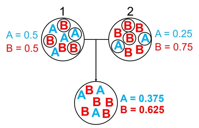
An example of the difference between allele frequency and identity.In this example (and many of the figures that follow in this post), the circle denote different populations, within which there are individuals which possess either an A gene (blue) or a B gene. Left: If we compared Populations 1 and 2, we can see that they both have A and B alleles. However, these alleles vary in their frequency within each population, with an equal balance of A and B in Pop 1 and a much higher frequency of B in Pop 2. Right: However, when we compared Pop 3 and 4, we can see that not only do they vary in frequencies, they vary in the presence of alleles, with one allele in each population but not the other.
An example of how gene flow across populations homogenises allele frequencies. We start with two initial populations (1 and 2 from above), which have very different allele frequencies. Hybridising individuals across the two populations means some alleles move from Pop 1 and Pop 2 into the hybrid population: which alleles moves is random (the smaller circles). Because of this, the resultant hybrid population has an allele frequency somewhere in between the two source populations: think of like mixing red and blue cordial and getting a purple drink.
An example of a Structure plot which long-term The G-CAT readers may be familiar with. This is taken from Brauer et al. (2013), where the authors studied the population structure of the Yarra pygmy perch. Each small column represents a single individual, with the colours representing how well the alleles of that individual fit a particular genetic population (each population has one colour). The numbers and broader columns refer to different ‘localities’ (different from populations) where individuals were sourced. This shows clear strong population structure across the 4 main groups, except for in Locality 6 where there is a mixture of Eastern and Merri/Curdies alleles.
Determining genetic bottlenecks and demographic change
A diagram of how allele frequencies change in genetic bottlenecks due to genetic drift. Left: Large circles again denote a population (although across different sequential times), with smaller circle denoting which alleles survive into the next generation (indicated by the coloured arrows). We start with an initial ‘large’ population of 8, which is reduced down to 4 and 2 in respective future times. Each time the population contracts, only a select number of alleles (or individuals) ‘survive’: assuming no natural selection is in process, this is totally random from the available gene pool. Right: We can see that over time, the frequencies of alleles A and B shift dramatically, leading to the ‘extinction’ of Allele B due to genetic drift. This is because it is the less frequent allele of the two, and in the smaller population size has much less chance of randomly ‘surviving’ the purge of the genetic bottleneck.
An example of how the frequency of alleles might vary under natural selection in correlation to the environment. In this example, the blue allele A is adaptive and under positive selection in the more intense environment, and thus increases in frequency at higher values. Contrastingly, the red allele B is maladaptive in these environments and decreases in frequency. For comparison, the black allele shows how the frequency of a neutral (non-adaptive or maladaptive) allele doesn’t vary with the environment, as it plays no role in natural selection.
Fixed differences are sometimes used as a type of diagnostic trait for species. This means that each ‘species’ has genetic variants that are not shared at all with its closest relative species, and that these variants are so strongly under selection that there is no diversity at those loci. Often, fixed differences are considered a level above populations that differ by allelic frequency only as these alleles are considered ‘diagnostic’ for each species.
An example of the difference between fixed differences and allelic frequency differences. In this example, we have 5 cats from 3 different species, sequencing a particular target gene. Within this gene, there are three possible alleles: T, A or G respectively. You’ll quickly notice that the T allele is both unique to Species A and is present in all cats of that species (i.e. is fixed). This is a fixed difference between Species A and the other two. Alleles A and G, however, are present in both Species B and C, and thus are not fixed differences even if they have different frequencies.
To distinguish between the two, we often use the overall frequency of alleles in a population as a basis for determining how likely two individuals share an allele by random chance. If alleles which are relatively rare in the overall population are shared by two individuals, we expect that this similarity is due to family structure rather than population history. By factoring this into our relatedness estimates we can get a more accurate overview of how likely two individuals are to be related using genetic information.
The wild world of allele frequency
Despite appearances, this is just a brief foray into the many applications of allele frequency data in evolution, ecology and conservation studies. There are a plethora of different programs and methods that can utilise this information to address a variety of scientific questions and refine our investigations.
Meaning: Cinis: from [ash] in Latin; descendens from [descends] in Latin.
Translation: descending from the ash; describes hunting behaviour in ash mountains of Vvardenfell.
Common name
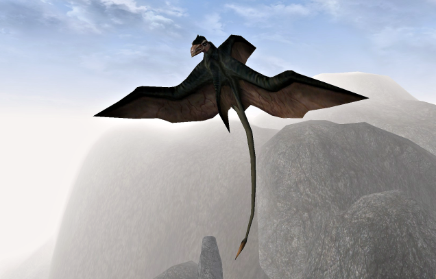
Cliff racer
A cliff racer hovering above a precipice on Vvardenfell.
Taxonomic status
Kingdom Animalia; Phylum Chordata; Class Aves; Subclass Archaeornithes; Family Vvardidae; GenusCinis; Speciesdescendens
Conservation status
Least Concern [circa 3E 427]
Threatened [circa 4E 433]
Distribution
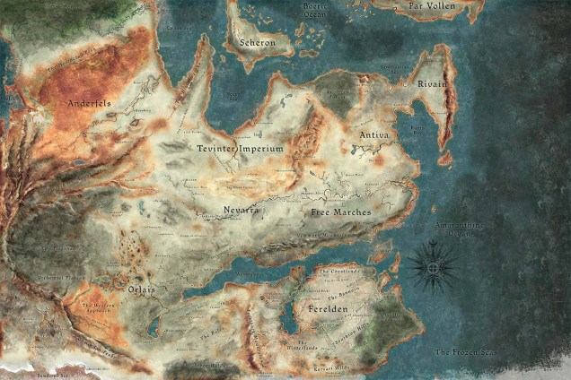
Once widespread throughout the north eastern region of Tamriel, occupying regions from the island of Vvardenfell to mainland Morrowind and Solstheim. Despite their name, the cliff racer is found across nearly all geographic regions of Vvardenfell, although the species is found in greatest densities in the rocky interior region of Stonefalls.
Following a purge of the species as part of pest control management, the cliff racer was effectively exterminated from parts of its range, including local extinction on the island of Solstheim. Since the cull the cliff racer is much less abundant throughout its range although still distributed throughout much of Vvardenfell and mainland Morrowind.
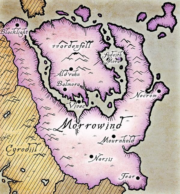
The province of Morrowind, which largely contains the distribution of the cliff racer. The island of Solstheim is found to the northwest of the map (the lower half of the island can be seen in brown).
Habitat
Although, much as the name suggests, the cliff racer prefers rocky outcroppings and mountainous regions in which it can build its nest, the species is frequently seen in lowland swamp and plains regions of Morrowind.
Behaviour and ecology
The cliff racer is a highly aggressive ambush predator, using height and range to descend on unsuspecting victims and lashing at them with its long, sharp tail. Although preferring to predate on small rodents and insects (such as kwama), cliff racers have been known to attack much larger beasts such as agouti and guar if provoked or desperate. The highly territorial nature of cliff racer means that they often attack travellers, even if they pose no immediate threat or have done nothing to provoke the animal.
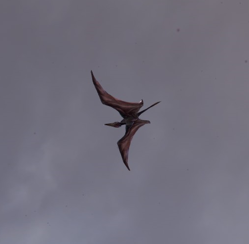
A cliff racer descends upon its prey.
Despite the territoriality of cliff racers, large flocks of them can often be found in the higher altitude regions of Vvardenfell, perhaps facilitated by an abundance of food (reducing competition) or communal breeding grounds. Attempts by researchers to study these aggregations have been limited due to constant attacks and damage to equipment by the flock.
Following the control measures implemented, the population size of these populations of cliff racers declined severely; however, given the survival of the majority of the population it does not appear this bottleneck has severely impacted the longevity of the species. The extirpation of the Solstheim population of cliff racers likely removed a unique ESU from the species, given the relative isolation of the island. Whether the island will be recolonised in time by Vvardenfell cliff racers is unknown, although the presence of any cliff racers back onto Solstheim would likely be met with strong opposition from the local peoples.
Adaptive traits
The broad wings, dorsal sail and long tail allow the cliff racer to travel large distances in the air, serving them well in hunting behaviour. The drawback of this is that, if hunting during the middle hours of the day, the cliff racer leaves an imposing shadow on the ground and silhouette in the sky, often alerting aware prey to their presence. That said, the speed of descent and disorienting cry of the animal often startles prey long enough for the cliff racer to attack.
The plumes of the cliff racer are a well-sought-after commodity by local peoples, used in the creation of garments and household items. Whether these plumes serve any adaptive purpose (such as sexual selection through mate signalling) is unknown, given the difficulties with studying wild cliff racer behaviour.
Management actions
Although suffering from a strong population bottleneck after the purge, the cliff racer is still relatively abundant across much of its range and maintains somewhat stable size. Management and population control of the cliff racer is necessary across the full distribution of the species to prevent strong recovery and maintain public safety and ecosystem balance. Breeding or rescuing cliff racers is strictly forbidden and the species has been widely declared as ‘native pest’, despite the somewhat oxymoron nature of the phrase.
Nugs are non-confrontational omnivorous species, preferring to hide and delve in the dark underground systems below the world of Thedas. Thus, nugs will typically avoid contact with people or predators by hiding in various crevices, using their pale skin to blend in with the surrounding rock faces. Reports of nugs in the wild demonstrate that nugs are remarkably inefficient at predator avoidance, despite their physiology; however, nug populations do not appear to suffer dramatically with predator presence, suggesting that either predators are too few to significantly impact population size or that alternative behaviours might allow them to rapidly bounce back from natural declines.
Given the lack of consistent light within their habitat, nugs are effectively blind, retaining only limited eyesight required for moving around above the surface. Nugs feed on a large variety of food sources, preferring insects but resorting to mineral deposits if available food resources are depleted. Their generalist diet may be one physiological trait that has allowed the nug to become some widespread and abundant historically.
Demography
Although the nug is a widespread and abundant species, they are heavily reliant on the connections of the Deep Roads to maintain connectivity and gene flow. With the gradual declination of Dwarven abundance and the loss of entire regions of the underground civilisation, it is likely that many areas of the nug distribution have become isolated and suffering from varying levels of inbreeding depression. Given the lack of access to these populations, whether some have collapsed since their isolation is unknown and potentially isolated populations may have even speciated if local environments have changed significantly.
Adaptive traits
Nugs are highly adapted to low-light, subterranean conditions, and show many phenotypic traits related to this kind of environment. The reduction of eyesight capability is considered a regression of unusable traits in underground habitats; instead, nugs show a highly developed and specialised nasal system. The high sensitivity of the nasal cavity makes them successful forages in the deep caverns of the underworld, and the elongated maw of the nug allows them to dig into buried food sources with ease. One of the more noticeable (and often disconcerting) traits of the nug is their human-like hands; the development of individual digits similar to fingers allows the nug to grip and manipulate rocky surfaces with surprising ease.
Management actions
Re-establishment of habitat corridors through the clearing and revival of the Deep Roads is critical for both reconnecting isolated populations of nugs and restoring natural gene flow, but also allowing access to remote populations for further studies. A combination of active removal of resident Darkspawn and population genetics analysis to accurately assess the conservation status of the species. That said, given the commercial value of the nug as a food source for many societies, establishing consistent sustainable farming practices may serve to both boost the nug populations and also provide an industry for many people.