Biological Species Concept

The folly of absolute dichotomies

November 21, 2018thegcatblog4 Comments

Divide and conquer (nothing)

Divisiveness is becoming quickly apparent as a plague on the modern era. The segregation and categorisation of people – whether politically, spiritually or morally justified – permeates throughout the human condition and in how we process the enormity of the Homo sapien population. The idea that the antithetic extremes form two discrete categories (for example, the waning centrist between ‘left’ vs. ‘right’ political perspectives) is widely employed in many aspects of the world.

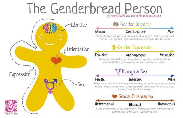
But how pervasive is this pattern? How well can we summarise, divide and categorise people? For some things, this would appear innately very easy to do – one of the most commonly evoked divisions in people is that between men and women. But the increasingly charged debate around concepts of both gender and sex (and sexuality as a derivative, somewhat interrelated concept) highlights the inconsistency of this divide.

The ‘sex’ and ‘gender’ arguments

The most commonly used argument against ‘alternative’ concepts of either gender of sex – the binary states of a ‘man’ with a ‘male’ body and a ‘female’ with a ‘female’ body – is often based on some perception of “biologically reality.” As a (trainee) biologist, let me make this apparently clear that such confidence and clarity of “reality” in many, if not all, biological subdisciplines is absurd (e.g. “nature vs. nurture”). Biologists commonly acknowledge (and rely upon) the realisation that life in all of its constructs is unfathomably diverse, unique, and often difficult to categorise. Any impression of being able to do so is a part of the human limitation to process concepts without boundaries.

Genderbread-Person figure — A great example of the complex nature of human sex and gender. You’ll notice that each category is itself a spectrum: even Biological Sex is not a clearly binary system. In fact, even this representation likely simplifies the complexity of human identity and sexuality given that each category is only a single linear scale (e.g. pansexuality and asexuality aren’t on the Sexual Orientation gradient), but nevertheless is a good summary. Source: It’s Pronounced METROsexual.

Gender as a binary

In terms of gender identity, I think this is becoming (slowly) more accepted over time. That most people have a gender identity somewhere along a multidimensional spectrum is not, for many people, a huge logical leap. Trans people are not mentally ill, not all ‘men’ identify as ‘men’ and certainly not all ‘men’ identify as a ‘man’ under the same characteristics or expression. Human psychology is beautifully complex and to reduce people down to the most simplistic categories is, in my humble opinion, a travesty. The single-variable gender binary cannot encapsulate the full depth of any single person’s identity or personality, and this biologically makes sense.

Sex as a binary

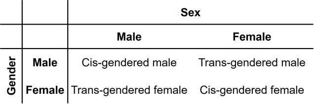
As an extension of the gender debate, sex itself has often been relied upon as the last vestige of some kind of sexual binary. Even for those more supported of trans people, sex is often described as some concrete, biologically, genetically-encoded trait which conveniently falls into its own binary system. Thus, instead of a single binary, people are reduced down to a two-character matrix of sex and gender.

Gender and sex table.jpg — A representative table of the “2 Character Sex and Gender” composition. Although slightly better at allowing for complexity in people’s identities, having 2 binaries instead of 1 doesn’t encapsulate the full breadth of diversity in either sex or gender.

However, the genetics of the definition and expression of sex is in itself a complex network of the expression of different genes and the presence of different chromosomes. Although high-school level biology teaches us that men are XY and women are XX genetically, individual genes within those chromosomes can alter the formation of different sexual organs and the development of a person. Furthermore, additional X or Y chromosomes can further alter the way sexual development occurs in people. Many people who fall in between the two ends of the gender spectrum of Male and Female identify as ‘intersex’.

DSD types table.jpg — A list of some of the known types of ‘Disorders of Sex Development’ (DSDs) which can lead to non-binary sex development in many different ways. Within these categories, there may be multiple genetic mechanisms (e.g. specific mutations) underlying the symptoms. It’s also important to note that while DSD medically describes the conditions of many people, it can be offensive/inappropriate to many intersex people (‘disorder’ can be a heavy word). Source: El-Sherbiny (2013).

You might be under the impression that these are rare ‘genetic disorders’, and don’t count as “real people” (decidedly not my words). But the reality is that intersex people are relatively common throughout the world, and occur roughly as frequently as true redheads or green eyes. Thus, the idea that excluding intersex people from the rest of societal definitions has very little merit, especially from a scientific point of view. Instead, allowing our definitions of both sex and gender to be broad and flexible allows us to incorporate the biological reality of the immense diversity of the world, even just within our own species.

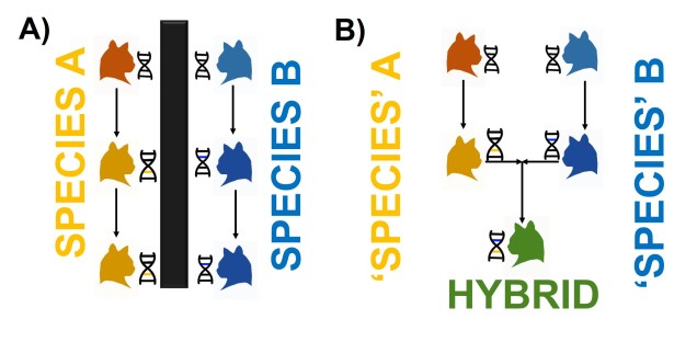
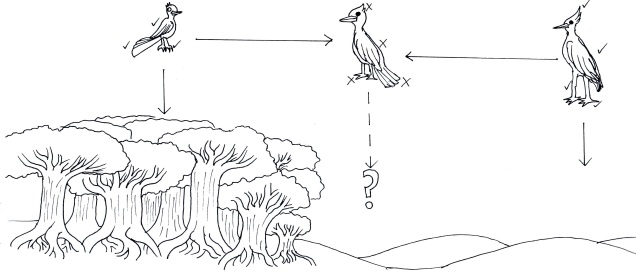
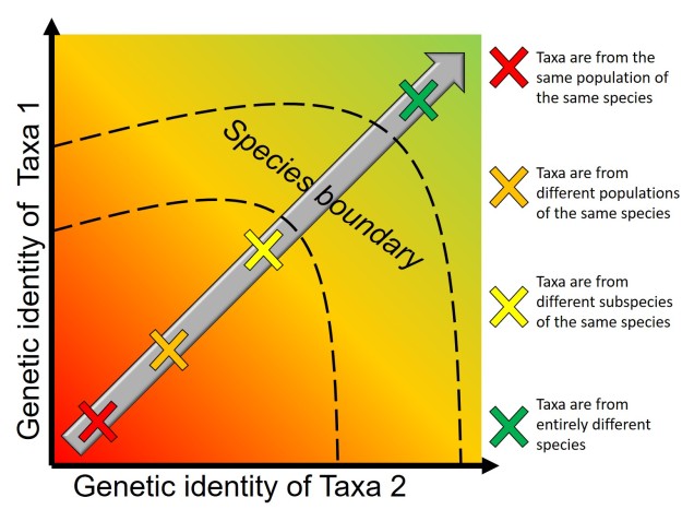
Absolute species concepts

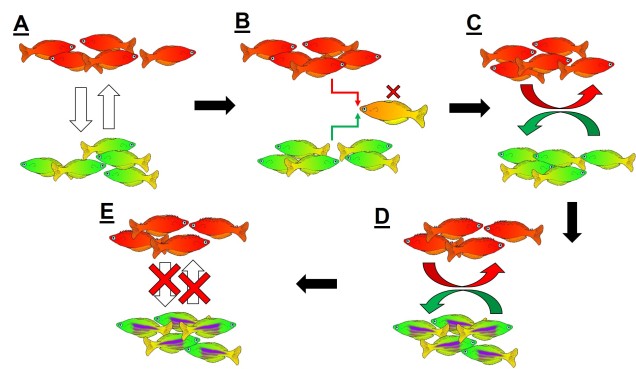
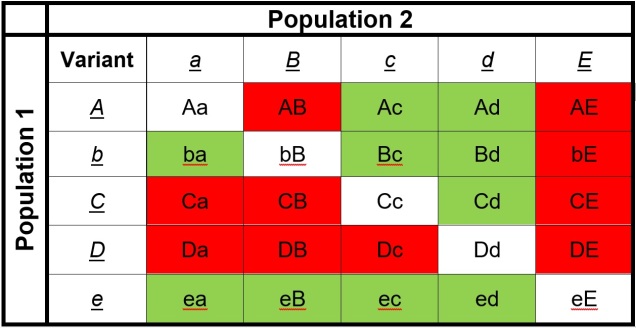
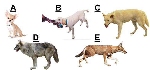
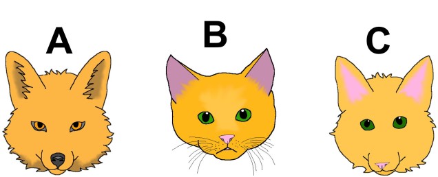
Speaking of species, and relating this paradigm of dichotomy to potentially less politically charged concepts, species themselves are a natural example on the inaccuracy of absolutism. This idea is not a new one, either within The G-CAT or within the broad literature, and species identity has long been regarded as a hive of grey areas. The sheer number of ways a group of organisms can be divided into species (or not, as the case may be) lends to the idea that simplified definitions of what something is or is not will rarely be as accurate as we hope. Even the most commonly employed of characteristics – such as those of the Biological Species Concept – cannot be applied to a number of biological systems such as asexually-reproducing species or complex cases of isolation.

Speciation continuum figure — A figure describing the ‘speciation continuum’ from a previous post on The G-CAT. Now imagine that each Species Concept has it’s own vague species boundary (dotted line): draw 30 of them over the top of one another, and try to pick the exact cut-off between the red and green areas. Even using the imagination, this would be difficult.

The diversity of Life

Anyone who argues a biological basis for these concepts is taking the good name of biological science hostage. Diversity underpins the most core aspects of biology (e.g. evolution, communities and ecosystems, medicine) and is a real attribute of living in a complicated world. Downscaling and simplifying the world to the ‘black’ and the ‘white’ discredits the wonder of biology, and acknowledging the ‘outliers’ (especially those that are not actually so far outside the boxes we have drawn) of any trends we may observe in nature is important to understand the complexity of life on Earth. Even if individual components of this post seem debatable to you: always remember that life is infinitely more complex and colourful than we can even imagine, and all of that is underpinned by diversity in one form or another.

An identity crisis: using genomics to determine species identities

July 18, 2018thegcatblog6 Comments

This is the fourth (and final) part of the miniseries on the genetics and process of speciation. To start from Part One, click here.

In last week’s post, we looked at how we can use genetic tools to understand and study the process of speciation, and particularly the transition from populations to species along the speciation continuum. Following on from that, the question of “how many species do I have?” can be further examined using genetic data. Sometimes, it’s entirely necessary to look at this question using genetics (and genomics).

Cryptic species

A concept that I’ve mentioned briefly previously is that of ‘cryptic species’. These are species which are identifiable by their large genetic differences, but appear the same based on morphological, behavioural or ecological characteristics. Cryptic species often arise when a single species has become fragmented into several different populations which have been isolated for a long time from another. Although they may diverge genetically, this doesn’t necessarily always translate to changes in their morphology, ecology or behaviour, particularly if these are strongly selected for under similar environmental conditions. Thus, we need to use genetic methods to be able to detect and understand these species, as well as later classify and describe them.

Cryptic species heatmap example — The level of genetic differentiation between the fish in the above example. The phylogenies on the left and top of the figure demonstrate the evolutionary relationships of these four fish. The matrix shows a heatmap of the level of differences between different pairwise comparisons of all four fish: red squares indicate zero genetic differences (such as when comparing a fish to itself; the middle diagonal) whilst yellow squares indicate increasingly higher levels of genetic differentiation (with bright yellow = all differences). By comparing the different fish together, we can see that Fish 1 and 2, and Fish 3 and 4, are relatively genetically similar to one another (red-deep orange). However, other comparisons show high level of genetic differences (e.g. 1 vs 3 and 1 vs 4). Based on this information, we might suggest that Fish 1 and 2 belong to one cryptic species (A) and Fish 3 and 4 belong to a second cryptic species (B).

Genetic tools to study species: the ‘Barcode of Life’

A classically employed method that uses DNA to detect and determine species is referred to as the ‘Barcode of Life’. This uses a very specific fragment of DNA from the mitochondria of the cell: the cytochrome c oxidase I gene, CO1. This gene is made of 648 base pairs and is found pretty well universally: this and the fact that CO1 evolves very slowly make it an ideal candidate for easily testing the identity of new species. Additionally, mitochondrial DNA tends to be a bit more resilient than its nuclear counterpart; thus, small or degraded tissue samples can still be sequenced for CO1, making it amenable to wildlife forensics cases. Generally, two sequences will be considered as belonging to different species if they are certain percentage different from one another.

Annotated mitogeome — The full (annotated) mitochondrial genome of humans, with the different genes within it labelled. The CO1 gene is labelled with the red arrow (sometimes also referred to as COX1) whilst blue arrows point to other genes often used in phylogenetic or taxonomic studies, depending on the group or species in question.

Despite the apparent benefits of CO1, there are of course a few drawbacks. Most of these revolve around the mitochondrial genome itself. Because mitochondria are passed on from mother to offspring (and not at all from the father), it reflects the genetic history of only one sex of the species. Secondly, the actual cut-off for species using CO1 barcoding is highly contentious and possibly not as universal as previously suggested. Levels of sequence divergence of CO1 between species that have been previously determined to be separate (through other means) have varied from anywhere between 2% to 12%. The actual translation of CO1 sequence divergence and species identity is not all that clear.

Gene tree – species tree incongruences

One particularly confounding aspect of defining species based on a single gene, and with using phylogenetic-based methods, is that the history of that gene might not actually be reflective of the history of the species. This can be a little confusing to think about but essentially leads to what we call “gene tree – species tree incongruence”. Different evolutionary events cause different effects on the underlying genetic diversity of a species (or group of species): while these may be predictable from the genetic sequence, different parts of the genome might not be as equally affected by the same exact process.

A classic example of this is hybridisation. If we have two initial species, which then hybridise with one another, we expect our resultant hybrids to be approximately made of 50% Species A DNA and 50% Species B DNA (if this is the first generation of hybrids formed; it gets a little more complicated further down the track). This means that, within the DNA sequence of the hybrid, 50% of it will reflect the history of Species A and the other 50% will reflect the history of Species B, which could differ dramatically. If we randomly sample a single gene in the hybrid, we will have no idea if that gene belongs to the genealogy of Species A or Species B, and thus we might make incorrect inferences about the history of the hybrid species.

Gene tree incongruence figure — A diagram of gene tree – species tree incongruence. Each individual coloured line represents a single gene as we trace it back through time; these are mostly bound within the limits of species divergences (the black borders). For many genes (such as the **blue** ones), the genes resemble the pattern of species divergences very well, albeit with some minor differences in how long ago the splits happened (at the top of the branches). However, the **red** genes contrast with this pattern, with clear movement across species (from A and C into B): this represents genes that have been transferred by hybridisation. The **green** line represents a gene affected by what we call incomplete lineage sorting; that is, we cannot trace it back far enough to determine exactly how/when it initially diverged and so there are still two separate green lines at the very top of the figure. You can think of each line as a separate phylogenetic tree, with the overarching species tree as the **average pattern** of all of the genes.

There are a number of other processes that could similarly alter our interpretations of evolutionary history based on analysing the genetic make-up of the species. The best way to handle this is simply to sample more genes: this way, the effect of variation of evolutionary history in individual genes is likely to be overpowered by the average over the entire gene pool. We interpret this as a set of individual gene trees contained within a species tree: although one gene might vary from another, the overall picture is clearer when considering all genes together.

Species delimitation

In earlier posts on The G-CAT, I’ve discussed the biogeographical patterns unveiled by my Honours research. Another key component of that paper involved using statistical modelling to determine whether cryptic species were present within the pygmy perches. I didn’t exactly elaborate on that in that section (mostly for simplicity), but this type of analysis is referred to as ‘species delimitation’. To try and simplify complicated analyses, species delimitation methods evaluate possible numbers and combinations of species within a particular dataset and provides a statistical value for which configuration of species is most supported. One program that employs species delimitation is Bayesian Phylogenetics and Phylogeography (BPP): to do this, it uses a plethora of information from the genetics of the individuals within the dataset. These include how long ago the different populations/species separated; which populations/species are most related to one another; and a pre-set minimum number of species (BPP will try to combine these in estimations, but not split them due to computational restraints). This all sounds very complex (and to a degree it is), but this allows the program to give you a statistical value for what is a species and what isn’t based on the genetics and statistical modelling.

Vittata cryptic species — The cryptic species of pygmy perches identified within my research paper. This represents part of the main phylogenetic tree result, with the estimates of divergence times from other analyses included. The pictures indicate the physiology of the different ‘species’: Nannoperca pygmaea is morphologically different to the other species of Nannoperca vittata. Species delimitation analysis suggested all four of these were genetically independent species; at the very least, it is clear that there must be at least 2 species of Nannoperca vittata since A is more related to N. pygmaea than to other N. vittata species. Photo credits: N. vittata = Chris Lamin; N. pygmaea = David Morgan.

The end result of a BPP run is usually reported as a species tree (e.g. a phylogenetic tree describing species relationships) and statistical support for the delimitation of species (0-1 for each species). Because of the way the statistical component of BPP works, it has been found to give extremely high support for species identities. This has been criticised as BPP can, at time, provide high statistical support for genetically isolated lineages (i.e. divergent populations) which are not actually species.

Improving species identities with integrative taxonomy

Due to this particular drawback, and the often complex nature of species identity, using solely genetic information such as species delimitation to define species is extremely rare. Instead, we use a combination of different analytical techniques which can include genetic-based evaluations to more robustly assign and describe species. In my own paper example, we suggested that up to three ‘species’ of N. vittata that were determined as cryptic species by BPP could potentially exist pending on further analyses. We did not describe or name any of the species, as this would require a deeper delve into the exact nature and identity of these species.

As genetic data and analytical techniques improve into the future, it seems likely that our ability to detect and determine species boundaries will also improve. However, the additional supported provided by alternative aspects such as ecology, behaviour and morphology will undoubtedly be useful in the progress of taxonomy.

From mutation to speciation: the genetics of species formation

July 11, 2018July 11, 2018thegcatblog4 Comments

The genetics of speciation

Given the strong influence of genetic identity on the process and outcomes of the speciation process, it seems a natural connection to use genetic information to study speciation and species identities. There is a plethora of genetics-based tools we can use to investigate how speciation occurs (both the evolutionary processes and the external influences that drive it). One clear way to test whether two populations of a particular species are actually two different species is to investigate genes related to reproductive isolation: if the genetic differences demonstrate reproductive incompatibilities across the two populations, then there is strong evidence that they are separate species (at least under the Biological Species Concept; see Part One for why!). But this type of analysis requires several tools: 1) knowledge of the specific genes related to reproduction (e.g. formation of sperm and eggs, genital morphology, etc.), 2) the complete and annotated genome of the species (to be able to find and analyse the right genes properly) and 3) a good amount of data for the populations in question. As you can imagine, for people working on non-model species (i.e. ones that haven’t had the same history and detail of research as, say, humans and mice), this can be problematic. So, instead, we can use other genetic information to investigate and suggest patterns and processes related to the formation of new species.

Is reproductive isolation naturally selected for or just a consequence?

A fundamental aspect of studies of speciation is a “chicken or the egg”-type paradigm: does natural selection directly select for rapid reproductive isolation, preventing interbreeding; or as a secondary consequence of general adaptive differences, over a long history of evolution? This might be a confusing distinction, so we’ll dive into it a little more.

Of the two proposed models of speciation, the by-product of natural selection (the second model) has been the more favoured. Simply put, this expands on Darwin’s theory of evolution that describes two populations of a single species evolving independently of one another. As these become more and more different, both in physical (‘phenotype’) and genetic (‘genotype’) characteristics, there comes a turning point where they are so different that an individual from one population could not reasonably breed with an individual from the other to form a fertile offspring. This could be due to genetic incompatibilities (such as different chromosome numbers), physiological differences (such as changes in genital morphology), or behavioural conflicts (such as solitary vs. group living).

Certainly, this process makes sense, although it is debatable how fast reproductive isolation would occur in a given species (or whether it is predictable just based on the level of differentiation between two populations). Another model suggests that reproductive isolation actually might arise very quickly if natural selection favours maintaining particular combinations of traits together. This can happen if hybrids between two populations are not particularly well adapted (fit), causing natural selection to favour populations to breed within each group rather than across groups (leading to reproductive isolation). Typically, this is referred to as ‘reinforcement’ and predominantly involves isolating mechanisms that prevent individuals across populations from breeding in the first place (since this would be wasted energy and resources producing unfit offspring). The main difference between these two models is the sequence of events: do populations ecologically diverge, and because of that then become reproductively isolated, or do populations selectively breed (enforcing reproductive isolation) and thus then evolve independently?

Reinforcement figure.jpg — An example of reinforcement leading to speciation. A) We start with two populations of a single species (a red fish population and a green fish population), which can interbreed (the arrows). B) Because these two groups can breed, hybrids of the two populations can be formed. However, due to the poor combination of red and green fish genes within a hybrid, they are not overly fit (the red cross). C) Since natural selection doesn’t favour forming hybrids, populations then adapt to selectively breed only with similar fish, reducing the amount of interbreeding that occurs. D) With the two populations effectively isolated from one another, different adaptations specific to each population (spines in red fish, purple stripes in green fish) can evolve, causing them to further differentiate. E) At some point in the differentiation process, hybrids move from being just selectively unfit (as in B)) to entirely impossible, thus making the two populations formal species. In this example, evolution has directly selected against hybrids first, thus then allowing ecological differences to occur (as opposed to the other way around).

Reproductive isolation through DMIs

The reproductive incompatibility of two populations (thus making them species) is often intrinsically linked to the genetic make-up of those two species. Some conflicts in the genetics of Population 1 and Population 2 may mean that a hybrid having half Population 1 genes and half Population 2 genes will have serious fitness problems (such as sterility or developmental problems). Dramatic genetic differences, particularly a difference in the number of chromosomes between the two sources, is a significant component of reproductive isolation and is usually to blame for sterile hybrids such as ligers, zorse and mules.

However, subtler genetic differences can also have a strong effect: for example, the unique combination of Population 1 and Population 2 genes within a hybrid might interact with one another negatively and cause serious detrimental effects. These are referred to as “Dobzhansky-Müller Incompatibilities” (DMIs) and are expected to accumulate as the two populations become more genetically differentiated from one another. This can be a little complicated to imagine (and is based upon mathematical models), but the basis of the concept is that some combinations of gene variants have never, over evolutionary history, been tested together as the two populations diverge. Hybridisation of these two populations suddenly makes brand new combinations of genes, some of which may be have profound physiological impacts (including on reproduction).

DMI figure — An example of how Dobzhansky-Müller Incompatibilities arise, adapted from Coyne & Orr (2004). We start with an initial population (center top), which splits into two separate populations. In this example, we’ll look at how 5 genes (each letter = one gene) change over time in the separate populations, with the original allele of the gene (lowercase) occasionally mutating into a new allele (upper case). These mutations happen at random times and in random genes in each population (the red letters), such that the two become very different over time. After a while, these two populations might form hybrids; however, given the number of changes in each population, this hybrid might have some combinations of alleles that are ‘untested’ in their evolutionary history (see below). These untested combinations may cause the hybrid to be infertile or unviable, making the two populations isolated species.

DMI table — The list of ‘untested’ genetic combinations from the above example. This table shows the different combinations of each gene that could be made in a hybrid if these two populations interbred. The red cells indicate combinations that have never been ‘tested’ together; that is, at no point in the evolutionary history of these two populations were those two particular alleles together in the same individual. Green cells indicate ones that were together at some point, and thus are expected to be viable combinations (since the resultant populations are obviously alive and breeding).

How can we look at speciation in action?

We can study the process of speciation in the natural world without focussing on the ‘reproductive isolation’ element of species identity as well. For many species, we are unlikely to have the detail (such as an annotated genome and known functions of genes related to reproduction) required to study speciation at this level in any case. Instead, we might choose to focus on the different factors that are currently influencing the process of speciation, such as how the environmental, demographic or adaptive contexts of populations plays a role in the formation of new species. Many of these questions fall within the domain of phylogeography; particularly, how the historical environment has shaped the diversity of populations and species today.

Phylogeo of speciation — An example of the interplay between speciation and phylogeography, taken from Reyes-Velasco et al. (2018). They investigated the phylogeographic history of several different groups of species within the frog genus Ptychadena; in this figure, we can see how the different species (indicated by the colours and tree on the left) relate to the geography of their habitat (right).

A variety of different analytical techniques can be used to build a picture of the speciation process for closely related or incipient species. A good starting point for any speciation study is to look at how the different study populations are adapting; is there evidence that natural selection is pushing these populations towards different genotypes or ecological niches? If so, then this might be a precursor for speciation, and we can build on this inference with other complementary analyses.

For example, estimating divergence times between populations can help us suggest whether there has been sufficient time for speciation to occur (although this isn’t always clear cut). Additionally, we could estimate the levels of genetic hybridisation (‘introgression’) between two populations to suggest whether they are reasonably isolated and divergent enough to be considered functional species.

The future of speciation genomics

Although these can help answer some questions related to speciation, new tools are constantly needed to provide a clearer picture of the process. Understanding how and why new species are formed is a critical aspect of understanding the world’s biodiversity. How can we predict if a population will speciate at some point? What environmental factors are most important for driving the formation of new species? How stable are species identities, really? These questions (and many more) remain elusive for a wide variety of life on Earth.

What is a species, anyway?

June 27, 2018June 26, 2018thegcatblog9 Comments

This is Part 1 of a four part miniseries on the process of speciation; how we get new species, how we can see this in action, and the end results of the process. This week, we’ll start with a seemingly obvious question: what is a species?

The definition of a ‘species’

‘Species’ are a human definition of the diversity of life. When we talk about the diversity of life, and the myriad of creatures and plants on Earth, we often talk about species diversity. This might seem glaringly obvious, but there’s one key issue: what is a species, anyway? While we might like to think of them as discrete and obvious groups (a dog is definitely not the same species as a cat, for example), the concept of a singular “species” is actually the result of human categorisation.

In reality, the diversity of life is spread across a huge spectrum of differentiation: from things which are closely related but still different to us (like chimps), to more different again (other mammals), to hardly relatable at all (bacteria and plants). So, what is the cut-off for calling something a species, and not a different genus, family, or kingdom? Or alternatively, at what point do we call a specific sub-group of a species as a sub-species, or another species entirely?

This might seem like a simple question: we look at two things, and they look different, so they must be different species, right? Well, of course, nature is never simple, and the line between “different” and “not different” is very blurry. Here’s an example: consider that you knew nothing about the history, behaviour or genetics of dogs. If you simply looked at all the different breeds of dogs on Earth, you might suggest that there are hundreds of species of domestic dogs. That seems a little excessive though, right? In fact, the domestic dog, Eurasian wolf, and the Australian dingo are all the same species (but different subspecies, along with about 38 others…but that’s another issue altogether).

Dogs — Morphology can be misleading for identifying species. In this example, we have A) a dog, B) also a dog, C) still a dog, D) yet another dog, and E) not a dog. For the record, **A-D** are all Canis lupus of some variety; A and B are domestic dogs (Canis lupus familiaris), C is a dingo (Canis lupus dingo) and D is a grey wolf (Canis lupus lupus). E, however, is the Ethiopian wolf, Canis simensis.

How do we describe species?

This method of describing species based on how they look (their morphology) is the very traditional approach to taxonomy. And for a long time, it seemed to work…until we get to more complex scenarios like the domestic dog. Or scenarios where two species look fairly similar, but in reality have evolved entirely differently for a very, very long time. Or groups which look close to more than one other species. So how do we describe them instead?

Cats and foxes — A), a fox. B), a cat. C), a foxy cat? A catty fox? A cat-fox hybrid? Something unrelated to cat or a fox?

Believe it or not, there are dozens of ways of deciding what is a species and what isn’t. In Speciation (2004), Coyne & Orr count at least 25 different reported Species Concepts that had been suggested within science, based on different requirements such as evolutionary history, genetic identity, or ecological traits. These different concepts can often contradict one another about where to draw the line between species…so what do we use?

The Biological Species Concept (BSC)

The most commonly used species concept is called the Biological Species Concept (BSC), which denotes that “species are groups of interbreeding natural populations that are reproductively isolated from other such groups” (Mayr, 1942). In short, a population is considered a different species to another population if an individual from one cannot reliably breed to form fertile, viable offspring with an individual from the other. We often refer to this as “reproductive isolation.” It’s important to note that reproductive isolation doesn’t mean they can’t breed at all: just that the hybrid offspring will not live a healthy life and produce its own healthy offspring.

For example, a horse and zebra can breed to produce a zorse, however zorse are fundamentally infertile (due to the different number of chromosomes between a horse and a zebra) and thus a horse is a different species to a zebra. However, a German Shepherd and a chihuahua can breed and make a hybrid mutt, so they are the same species.

You might naturally ask why reproductive isolation is apparently so important for deciding species. Most directly, this means that groups don’t share gene pools at all (since genetic information is introduced and maintained over time through breeding events), which causes them to be genetically independent of one another. Thus, changes in the genetic make-up of one species shouldn’t (theoretically) transfer into the gene pool of another species through hybrids. This is an important concept as the gene pool of a species is the basis upon which natural selection and evolution act: thus, reproductively isolated species may evolve in very different manners over time.

RI example — An example of how reproductive isolation maintains genetic and evolutionary independence of species. In A), our cat groups are robust species, reproductively isolated from one another (as shown by the black box). When each species undergoes natural selection and their genetic variation changes (colour changes on the cats and DNA), these changes are kept within each lineage. This contrasts to B), where genetic changes can be transferred between species. Without reproductive isolation, evolution in the orange lineage and the blue lineage can combine within hybrids, sharing the evolutionary pathways of both ancestral species.

Pitfalls of the BSC

Just because the BSC is the most used concept doesn’t make it infallible, however. Many species on Earth don’t easily demonstrate reproductive isolation from one another, nor does the concept even make sense for asexually reproducing species. If an individual reproduced solely asexually (like many bacteria, or even some lizards), then by the BSC definition every individual is an entirely different species…which seems a little excessive. Even in sexually reproducing organisms, it can be hard to establish reproductive isolation, possibly because the species never come into contact physically.

This raises the debate of whether two species could, let alone will, hybridise in nature, which can be difficult to determine. And if two species do produce hybrid offspring, assessing their fertility or viability can be difficult to detect without many generations of breeding and measurements of fitness (hybrids may not be sustainable in nature if they are not well adapted to their environment and thus the two species are maintained as separate identities).

Hybrid birds — An example of unfit hybrids causing effective reproductive isolation. In this example, we have two different bird species adapted to very different habitats; a smaller, long-tailed bird (left) adapted to moving through dense forest, and a large, longer-legged bird (right) adapted to traversing arid deserts. When (or if) these two species hybridised, the resultant offspring would be middle of the road, possessing too few traits to be adaptive in either the forest or the desert and no fitting intermediate environment available. Measuring exactly how unfit this hybrid would be is a difficult task in establishing species boundaries.

Integrative taxonomy

To try and account for the issues with the BSC, taxonomists try to push for the usage of “integrative taxonomy”. This means that species should be defined by multiple different agreeing concepts, such as reproductive isolation, genetic differentiation, behavioural differences, and/or ecological traits. The more traits that can separate the two, the greater support there is for the species to be separated: if they disagree, then more information is needed to determine exactly whether or not that should be called different species. Debates about taxonomy are ongoing and are likely going to be relevant for years to come, but form critical components of understanding biodiversity, patterns of evolution, and creating effective conservation legislation to protect endangered or threatened species (for whichever groups we decide are species).

The G-cat

Dive head-first into the science of conservation, ecology, evolution and genetics