When I was younger, I used to love visiting our local creek: it was a beautiful spot of nature a short walk from home. On a couple occasions, my Dad took me to the creek to catch yabbies – for a suburban kid, it was one of the few times I actually held and interacted with wild biodiversity, and helped foster my love for conservation and inquiry into biology. In the late 2000s to early 2010s, a likely combination of local pollution and extensive drought extirpated the yabbies from the creek – I would never see one in that creek again. I was devastated for the local loss of a fascinating creature, and the connection to nature it represented, but felt powerless to remedy the situation. To my knowledge, there are still no yabbies in that creek.
Species which exist in fragmented, isolated and reduced populations have elevated extinction risk. Not only are they more susceptible to demographic and environmental stochasticity, which can easily wipe out small populations, but they also suffer from a range of genetic impacts. Notably, populations often lose significant amounts of genetic diversity as they reduce in size, potentially losing important adaptive diversity enabling them to respond to current and future environmental change. At the same time, random genetic drift becomes stronger relative to natural selection, reducing the efficacy of selection to be able to increase the frequency of favourable alleles and reduce the frequency of maladaptive ones. Together, these impacts create feedback loops which hasten the decline into the extinction vortex.
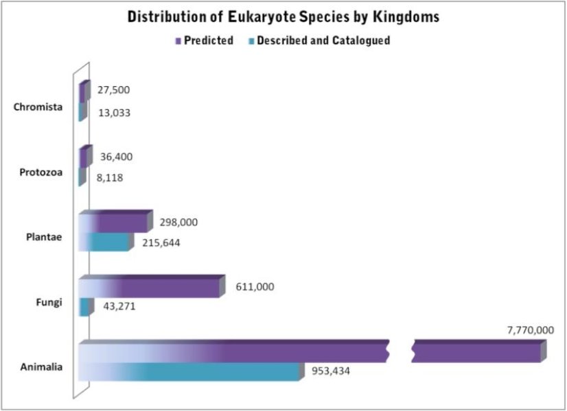
There are quite literally millions of species on Earth, ranging from the smallest of microbes to the largest of mammals. In fact, there are so many that we don’t actually have a good count on the sheer number of species and can only estimate it based on the species we actually know about. Unsurprisingly, then, the number of species vastly outweighs the number of people that research them, especially considering the sheer volumes of different aspects of species, evolution, conservation and their changes we could possibly study.
Some estimations on the number of eukaryotic species (i.e. not including things like bacteria), with the number of known species in blue and the predicted number of total species on Earth in purple. Source: Census of Marine Life.
This is partly where the concept of a ‘model’ comes into it: it’s much easier to pick a particular species to study as a target, and use the information from it to apply to other scenarios. Most people would be familiar with the concept based on medical research: the ‘lab rat’ (or mouse). The common house mouse (Mus musculus) and the brown rat (Rattus norvegicus) are some of the most widely used models for understanding the impact of particular biochemical compounds on physiology and are often used as the testing phase of medical developments before human trials.
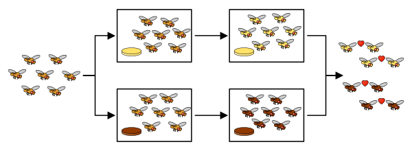
A simplified summary of the speciation experiment in Drosophila, starting with a single species and resulting in two reproductively isolated species based on mating and food preference. Source: Ilmari Karonen, adapted from here.
Some of Darwin’s early drawings of the morphological differences in Galapagos finch beaks, which lead to the formulation of the theory of evolution by natural selection.
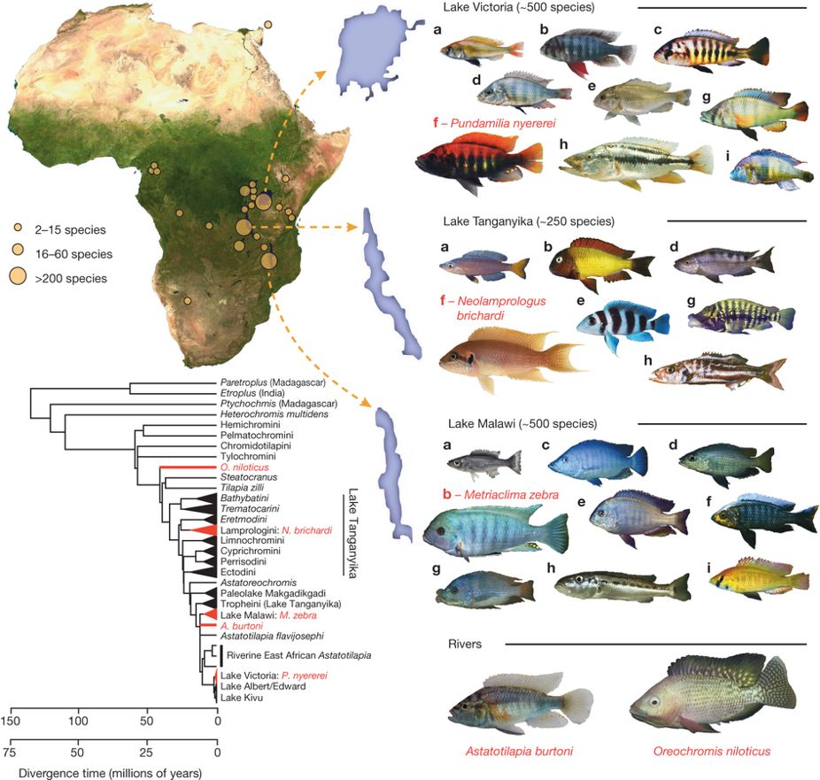
The sheer diversity of species and form makes African cichlids an ideal model for testing hypotheses and theories about the process of evolution and adaptive radiation. Figure sourced from Brawand et al. (2014) in Nature.
The idea of using the genetic sequences of living organisms to understand the evolutionary history of species is a concept much repeated on The G-CAT. And it’s a fundamental one in phylogenetics, taxonomy and evolutionary biology. Often, we try to analyse the genetic differences between individuals, populations and species in a tree-like manner, with close tips being similar and more distantly separated branches being more divergent. However, this runs on one very key assumption; that the patterns we observe in our study genes matches the overall patterns of species evolution. But this isn’t always true, and before we can delve into that we have to understand the difference between a ‘gene tree’ and a ‘species tree’.
A gene tree or a species tree?
Our typical view of a phylogenetic tree is actually one of a ‘gene tree’, where we analyse how a particular gene (or set of genes) have changed over time between different individuals (within and across populations or species) based on our understanding of mutation and common ancestry.
However, a phylogenetic tree based on a single gene only demonstrates the history of that gene. What we assume in most cases is that the history of that gene matches the history of the species: that branches in the genetic tree mirror when different splits in species occurred throughout history.
The easiest way to conceptualise gene trees and species trees is to think of individual gene trees that are nested within an overarching species tree. In this sense, individual gene trees can vary from one another (substantially, even) but by looking at the overall trends of many genes we can see how the genome of the species have changed over time.
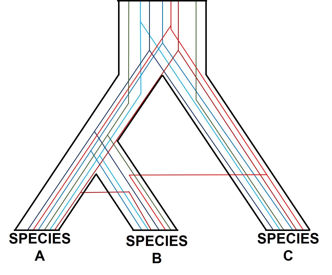
A (potentially familiar) depiction of individual gene trees (coloured lines) within the broader species tree (defined b the black boundaries). As you might be able to tell, the branching patterns of the different genes are not the same, and don’t always match the overarching species tree.
One of the most prolific, but more complicated, ways gene trees can vary from their overarching species tree is due to what we call ‘incomplete lineage sorting’. This is based on the idea that species and the genes that define them are constantly evolving over time, and that because of this different genes are at different stages of divergence between population and species. If we imagine a set of three related populations which have all descended from a single ancestral population, we can start to see how incomplete lineage sorting could occur. Our ancestral population likely has some genetic diversity, containing multiple alleles of the same locus. In a true phylogenetic tree, we would expect these different alleles to ‘sort’ into the different descendent populations, such that one population might have one of the alleles, a second the other, and so on, without them sharing the different alleles between them.
If this separation into new populations has been recent, or if gene flow has occurred between the populations since this event, then we might find that each descendent population has a mixture of the different alleles, and that not enough time has passed to clearly separate the populations. For this to occur, sufficient time for new mutations to occur and genetic drift to push different populations to differently frequent alleles needs to happen: if this is too recent, then it can be hard to accurately distinguish between populations. This can be difficult to interpret (see below figure for a visualisation of this), but there’s a great description of incomplete lineage sorting here.
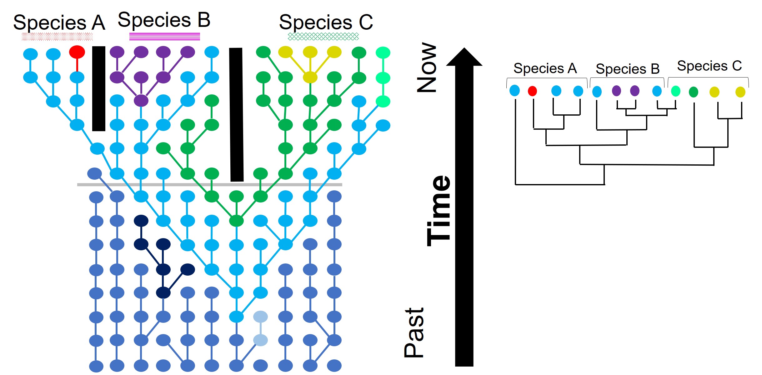
A demonstration of incomplete lineage sorting, generously adapted from a talk by fellow MELFU postdocs Dr Yuma (Jonathon) Sandoval-Castillo and Dr Catherine Attard. On the left is a depiction of a single gene coalescent tree over time: circles represent a single individual at a particular point in time (row) with the colours representing different alleles of that same gene. The tree shows how new mutations occur (colour changes along the branches) and spread throughout the descendent populations. In this example, we have three recently separated species, with a good number of different alleles. However, when we study these alleles in tree form (the phylogeny on the right), we see that the branches themselves don’t correlate well with the boundaries of the species. For example, the teal allele found within Species C is actually more similar to Species B alleles (purple and blue) than any other Species B alleles, based on the order and patterns of these mutations.
Hybridisation and horizontal transfer
Another way individual genes may become incongruent with other genes is through another phenomenon we’ve discussed before: hybridisation (or more specifically, introgression). When two individuals from different species breed together to form a ‘hybrid’, they join together what was once two separate gene pools. Thus, the hybrid offspring has (if it’s a first generation hybrid, anyway) 50% of genes from Species A and 50% of genes from Species B. In terms of our phylogenetic analysis, if we picked one gene randomly from the hybrid, we have 50% of picking a gene that reflects the evolutionary history of Species A, and 50% chance of picking a gene that reflects the evolutionary history of Species B. This would change how our outputs look significantly: if we pick a Species A gene, our ‘hybrid’ will look (genetically) very, very similar to Species A. If we pick a Species B gene, our ‘hybrid’ will look like a Species B individual instead. Naturally, this can really stuff up our interpretations of species boundaries, distributions and identities.
An example of hybridisation leading to gene tree incongruence with our favourite colourful fish. A) We have a hybridisation event between a red fish (Species A) and a green fish (Species B), resulting in a hybrid species (‘Species’ H). The red fish genome is indicated by the yellow DNA, the green fish genomes by the blue DNA, and the hybrid orange fish has a mixture of these two. B) If we sampled one set of genes in the hybrid, we might select a gene that originated from the red fish, showing that the hybrid is identical (or very similar) the Species A. D) Conversely, if we sampled a gene originating from the green fish, the resultant phylogeny might show that the hybrid is the same as Species B. C) If we consider these two patterns in combination, which see the true pattern of species formation, which is not a clear dichotomous tree and rather a mixture of the two sets of trees.
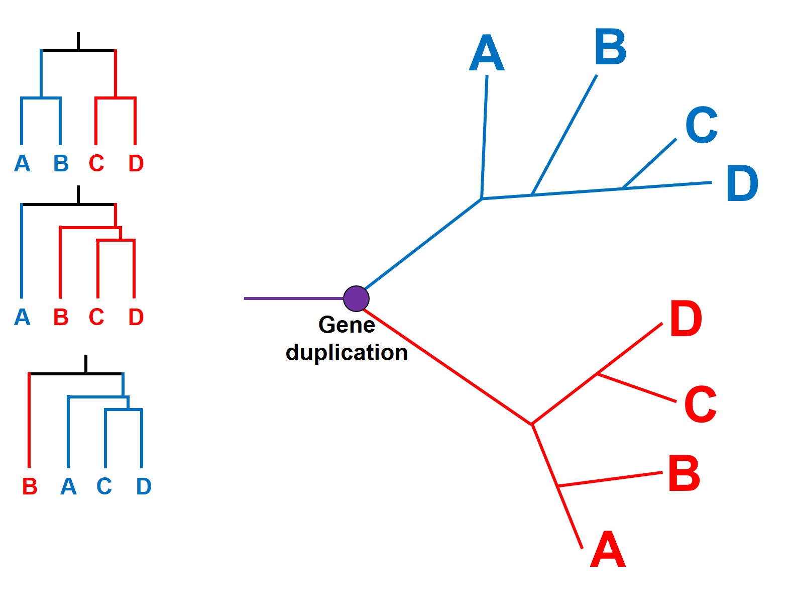
This can have a profound impact as paralogous genes are difficult to detect: if there has been a gene duplication early in the evolutionary history of our phylogenetic tree, then many (or all) of our study samples will have two copies of said gene. Since they look similar in sequence, there’s all possibility that we pick Variant 1 in some species and Variant 2 in other species. Being unable to tell them apart, we can have some very weird and abstract results within our tree. Most importantly, different samples with the same duplicated variant will seem similar to one another (e.g. have evolved from a common ancestor more recently) than it will to any sample of the other variant (even if they came from the exact same species)!
An example of how paralogous genes can confound species tree. We start with a single (purple) gene: at a particular point in time, this gene duplicates into a red and a blue form. Each of these genes then evolve and spread into four separate descendent species (A, B, C and D) but not in entirely the same way. However, since both the red and blue genetic sequences are similar, if we took a single gene from each species we might (somewhat randomly) sequence either the red or the blue copy. The different phylogenetic trees on the right demonstrate how different combinations of red and blue genes give very different patterns, since all blue copies will be more related to other blue genes than to the red gene of the same species. E.g. a blueA and a blueC are more similar than a blueA and a redA.
Overcoming incongruence with genomics
Although a tricky conundrum in phylogenetics and evolutionary genetics broadly, gene tree incongruence can largely be overcome with using more loci. As the random changes of any one locus has a smaller effect of the larger total set of loci, the general and broad patterns of evolutionary history can become clearer. Indeed, understanding how many loci are affected by what kind of process can itself become informative: large numbers of introgressed loci can indicate whether hybridisation was recent, strong, or biased towards one species over another, for example. As with many things, the genomic era appears poised to address the many analytical issues and complexities of working with genetic data.
Meaning: Octorokus from [octorok] in Hylian; infletus from [inflate] in Latin.
Translation: inflating octorok; all varieties use an inflatable air sac derived from the swim bladder to float and scan the horizon.
Varieties
Octorokus infletus hydros [aquatic morphotype]
Octorokus infletus petram [mountain morphotype]
Octorokus infletus silva [forest morphotype]
Octorokus infletus arctus [snow morphotype]
Octorokus infletus imitor [deceptive morphotype]
The various morphotypes of inflating octoroks. A: The water octorok, considered the morphotype closest to the ancestral physiology of the species. B: The forest octorok, with grass camouflage. C: The deceptive octorok, which has replaced its tufted vegetation with a glittering chest as bait. D: The mountainous octorok, with rock camouflage. E: The snow octorok, with tundra grass camouflage.
Common name
Variable octorok
Taxonomic status
Kingdom Animalia; Phylum Mollusca; Class Cephalapoda; Order Octopoda; Family Octopididae; GenusOctorokus; Speciesinfletus
Conservation status
Least Concern
Distribution
The species is found throughout all major habitat regions of Hyrule, with localised morphotypes found within specific habitats. The only major region where the variable octorok is not found is within the Gerudo Desert, suggesting some remnant dependency of standing water.
The region of Hyrule, with the distribution of octoroks in blue. The only major region where they are not found is the Gerudo Desert in the bottom left.
Habitat
Habitat choice depends on the physiology of the morphotype; so long as the environment allows the octorok to blend in, it is highly likely there are many around (i.e. unseen).
Behaviour and ecology
The variable octorok is arguably one of the most diverse species within modern Hyrule, exhibiting a large number of different morphotypic forms and occurring in almost all major habitat zones. Historical data suggests that the water octorok (Octorokus infletus hydros) is the most ancestral morphotype, with ancient literature frequently referring to them as sea-bearing or river-traversing organisms. Estimates from the literature suggests that their adaptation to land-based living is a recent evolutionary step which facilitated rapid morphological radiation of the lineage.
Several physiological characteristics unite the variable morphological forms of the octorok into a single identifiable species. Other than the typical body structure of an octopod (eight legs, largely soft body with an elongated mantle region), the primary diagnostic trait of the octorok is the presence of a large ‘balloon’ with the top of the mantle. This appears to be derived from the swim bladder of the ancestral octorok, which has shifted to the cranial region. The octorok can inflate this balloon using air pumped through the gills, filling it and lifting the octorok into the air. All morphotypes use this to scan the surrounding region to identify prey items, including attacking people if aggravated.
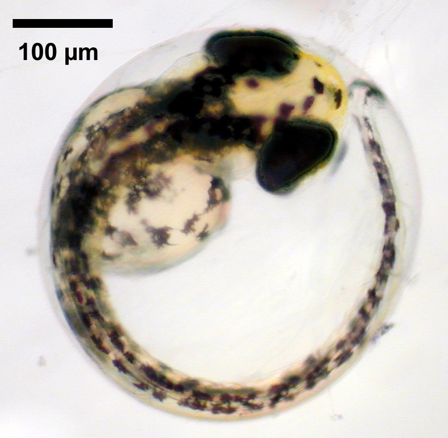
A water morphotype octorok with balloon inflated.
Diets of the octorok vary depending on the morphotype and based on the ecological habitat; adaptations to different ecological niches is facilitated by a diverse and generalist diet.
Demography
Although limited information is available on the amount of gene flow and population connectivity between different morphotypes, by sheer numbers alone it would appear the variable octorok is highly abundant. Some records of interactions between morphotypes (such as at the water’s edge within forested areas) implies that the different types are not reproductively isolated and can form hybrids: how this impacts resultant hybrid morphotypes and development is unknown. However, given the propensity of morphotypes to be largely limited to their adaptive habitats, it would seem reasonable to assume that some level of population structure is present across types.
Adaptive traits
The variable octorok appears remarkably diverse in physiology, although the recent nature of their divergence and the observed interactions between morphological types suggests that they are not reproductively isolated. Whether these are the result of phenotypic plasticity, and environmental pressures are responsible for associated physiological changes to different environments, or genetically coded at early stages of development is unknown due to the cryptic nature of octorok spawning.
All octoroks employ strong behavioural and physiological traits for camouflage and ambush predation. Vegetation is usually placed on the top of the cranium of all morphotypes, with the exact species of plant used dependent on the environment (e.g. forest morphotypes will use grasses or ferns, whilst mountain morphotypes will use rocky boulders). The octorok will then dig beneath the surface until just the vegetation is showing, effectively blending in with the environment and only occasionally choosing to surface by using the balloon. Whether this behaviour is passed down genetically or taught from parents is unclear.
Management actions
Few management actions are recommended for this highly abundant species. However, further research is needed to better understand the highly variable nature and the process of evolution underpinning their diverse morphology. Whether morphotypes are genetically hardwired by inheritance of determinant genes, or whether alterations in gene expression caused by the environmental context of octoroks (i.e. phenotypic plasticity) provides an intriguing avenue of insight into the evolution of Hylian fauna.
Nevertheless, the transition from the marine environment onto the terrestrial landscape appears to be a significant stepping stone in the radiation of morphological structures within the species. How this has been facilitated by the genetic architecture of the octorok is a mystery.