July 2018 – The G-cat

Moving right along: dispersal and population structure

July 25, 2018July 24, 2018thegcatblog9 Comments

The impact of species traits on evolution

Although we often focus on the genetic traits of species in molecular ecology studies, the physiological (or phenotypic) traits are equally as important in shaping their evolution. These different traits are not only the result themselves of evolutionary forces but may further drive and shape evolution into the future by changing how an organism interacts with the environment.

There are a massive number of potential traits we could focus on, each of which could have a large number of different (and interacting) impacts on evolution. One that is often considered, and highly relevant for genetic studies, is the influence of dispersal capability.

Dispersal

Dispersal is essentially the process of an organism migrating to a new habitat, to the point of the two being used almost interchangeably. Often, however, we regard dispersal as a migration event that actually has genetic consequences; particularly, if new populations are formed or if organisms move from one population to another. This can differ from straight migration in that animals that migrate might not necessarily breed (and thus pass on genes) into a new region during their migration; thus, evidence of those organisms will not genetically proliferate into the future through offspring.

Naturally, the ability of organisms to disperse is highly variable across the tree of life and reliant on a number of other physiological factors. Marine mammals, for example, can disperse extremely far throughout their lifetimes, whereas some very localised species like some insects may not move very far within their lifetime at all. The movement of organisms directly facilitates the movement of genetic material, and thus has significant impacts on the evolution and genetic diversity of species and populations.

Dispersal vs pop structure — The (simplistic) relationship between dispersal capability and one aspect of population genetics, population structure (measured as Fst). As organisms are more capable of dispersing longer distance (or more frequently), the barriers between populations become weaker.

Highly dispersive species

At one end of the dispersal spectrum, we have highly dispersive species. These can move extremely long distances and thus mix genetic material from a wide range of habitats and places into one mostly-cohesive population. Because of this, highly dispersive species often have strong colonising abilities and can migrate into a range of different habitats by tolerating a wide range of conditions. For example, a single whale might hang around Antarctica for part of the year but move to the tropics during other times. Thus, this single whale must be able to tolerate both ends of the temperature spectrum.

As these individuals occupy large ranges, localised impacts are unlikely to critically affect their full distribution. Individual organisms that are occupying an unpleasant space can easily move to a more favourable habitat (provided that one exists). Furthermore, with a large population (which is more likely with highly dispersive species), genetic drift is substantially weaker and natural selection (generally) has a higher amount of genetic diversity to work with. This is, of course, assuming that dispersal leads to a large overall population, which might not be the case for species that are critically endangered (such as the cheetah).

Highly dispersive animals often fit the “island model” of Wright, where individual subpopulations all have equal proportions of migrants from all other subpopulations. In reality, this is rare (or unreasonable) due to environmental or physiological limitations of species; distance, for example, is not implicitly factored into the basic island model.

Intermediately dispersing species

A large number of species, however, are likely to occupy a more intermediate range of dispersal ability. These species might be able to migrate to neighbouring populations, or across a large proportion of their geographic range, but individuals from one end of the range are still somewhat isolated from individuals at the other end.

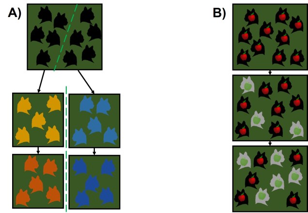
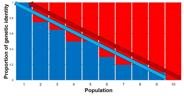
This often leads to some effect of population structure; different portions of the geographic range are genetically segregated from one another depending on how much gene flow (i.e. dispersal) occurs between populations. In the most simplest scenario, this can lead to what we call isolation-by-distance. Rather than forming totally independent populations, gene flow occurs across short ranges between adjacent ‘populations’. This causes a gradient of genetic differentiation, with one end of the range being clearly genetically different to the other end, with a gradual slope throughout the range. We see this often in marine invertebrates, for example, which might have somewhat localised dispersal but still occupy a large range by following oceanographic currents.

River IDB network — An example of how an isolation-by-distance population network might come about. In this example, we have a series of populations (the different pie charts) spread throughout a river system (that blue thing). The different pie charts represent how much of the genetics of that population matches one end of the river: either the blue end (left) or red end (right). Populations can easily disperse into adjacent populations (the green arrows) but less so to further populations. This leads to gradual changes across the length of the river, with the far ends of the river clearly genetically distinct from the opposite end but relatively similar to neighbouring populations.

River IDB pop structure.jpg — The genetic representation of the above isolation-by-distance example. Each column represents a single population (in the previous figure, a pie chart), with the different colours also representing the relative genetic identity of that population. As you can see, moving from Population 1 to 10 leads to a gradient (decreasing) in blue genes but increase in red genes. The inverse can be said moving in the opposite direction. That said, comparing Population 1 and Population 10 shows that they’re clearly different, although there is no clear cut-off point across the range of other populations.

Medium dispersal capabilities are also often a requirement for forming ‘metapopulations’. In this population arrangement, several semi-independent populations are present within the geographic range of the species. Each of these are subject to their own local environmental pressures and demographic dynamics, and because of this may go locally extinct at any given time. However, dispersal connections between many of these populations leads to recolonization and gene flow patterns, allowing for extinction-dispersal dynamics to sustain the overall metapopulation. Generally, this would require greater levels of dispersal than those typically found within metapopulation species, as individuals must traverse uninhabitable regions relatively frequently to recolonise locally extinct habitat.

Metapopulation structure.jpg — An example of metapopulation dynamics. Different subpopulations (lettered circles) are connected via dispersal (arrows). These different subpopulations can be different sizes and are mostly independent of one another, meaning that a single subpopulation can go locally extinct (the red X) without collapsing the entire system. The different dispersal pathways mean that one population can recolonise extinct habitat and essentially ‘rebirth’ other subpopulations (the green arrows).

Weakly dispersing species

At the far opposite end of the dispersal ability spectrum, we have low dispersal species. These are often localised, endemic species that for various reasons might be unable to travel very far at all; for some, they may spend their entire adult life in a sedentary form. The lack of dispersal lends to very strong levels of population structure, and individual populations often accumulate genetic differences relatively quickly due to genetic drift or local adaptation.

Species with low dispersal capabilities are often at risk of local extinction and are unable to easily recolonise these habitats after the event has ended. Their movement is often restricted to rare environmental events such as flooding that carry individuals long distances despite their physiological limitations. Because of this, low dispersal species are often at greater risk of total extinction and extinction vertices than their higher dispersing counterparts.

Accounting for dispersal in population genetics

Incorporating biological and physiological aspects of our study taxa is important for interpreting the evolutionary context of species. Dispersal ability is but one of many characteristics that can influence the ability of species to respond to selective pressures, and the context in which this natural selection occurs. Thus, understanding all aspects of an organism is important in building the full picture of their evolution and future prospects.

An identity crisis: using genomics to determine species identities

July 18, 2018thegcatblog6 Comments

This is the fourth (and final) part of the miniseries on the genetics and process of speciation. To start from Part One, click here.

In last week’s post, we looked at how we can use genetic tools to understand and study the process of speciation, and particularly the transition from populations to species along the speciation continuum. Following on from that, the question of “how many species do I have?” can be further examined using genetic data. Sometimes, it’s entirely necessary to look at this question using genetics (and genomics).

Cryptic species

A concept that I’ve mentioned briefly previously is that of ‘cryptic species’. These are species which are identifiable by their large genetic differences, but appear the same based on morphological, behavioural or ecological characteristics. Cryptic species often arise when a single species has become fragmented into several different populations which have been isolated for a long time from another. Although they may diverge genetically, this doesn’t necessarily always translate to changes in their morphology, ecology or behaviour, particularly if these are strongly selected for under similar environmental conditions. Thus, we need to use genetic methods to be able to detect and understand these species, as well as later classify and describe them.

Cryptic species heatmap example — The level of genetic differentiation between the fish in the above example. The phylogenies on the left and top of the figure demonstrate the evolutionary relationships of these four fish. The matrix shows a heatmap of the level of differences between different pairwise comparisons of all four fish: red squares indicate zero genetic differences (such as when comparing a fish to itself; the middle diagonal) whilst yellow squares indicate increasingly higher levels of genetic differentiation (with bright yellow = all differences). By comparing the different fish together, we can see that Fish 1 and 2, and Fish 3 and 4, are relatively genetically similar to one another (red-deep orange). However, other comparisons show high level of genetic differences (e.g. 1 vs 3 and 1 vs 4). Based on this information, we might suggest that Fish 1 and 2 belong to one cryptic species (A) and Fish 3 and 4 belong to a second cryptic species (B).

Genetic tools to study species: the ‘Barcode of Life’

A classically employed method that uses DNA to detect and determine species is referred to as the ‘Barcode of Life’. This uses a very specific fragment of DNA from the mitochondria of the cell: the cytochrome c oxidase I gene, CO1. This gene is made of 648 base pairs and is found pretty well universally: this and the fact that CO1 evolves very slowly make it an ideal candidate for easily testing the identity of new species. Additionally, mitochondrial DNA tends to be a bit more resilient than its nuclear counterpart; thus, small or degraded tissue samples can still be sequenced for CO1, making it amenable to wildlife forensics cases. Generally, two sequences will be considered as belonging to different species if they are certain percentage different from one another.

Annotated mitogeome — The full (annotated) mitochondrial genome of humans, with the different genes within it labelled. The CO1 gene is labelled with the red arrow (sometimes also referred to as COX1) whilst blue arrows point to other genes often used in phylogenetic or taxonomic studies, depending on the group or species in question.

Despite the apparent benefits of CO1, there are of course a few drawbacks. Most of these revolve around the mitochondrial genome itself. Because mitochondria are passed on from mother to offspring (and not at all from the father), it reflects the genetic history of only one sex of the species. Secondly, the actual cut-off for species using CO1 barcoding is highly contentious and possibly not as universal as previously suggested. Levels of sequence divergence of CO1 between species that have been previously determined to be separate (through other means) have varied from anywhere between 2% to 12%. The actual translation of CO1 sequence divergence and species identity is not all that clear.

Gene tree – species tree incongruences

One particularly confounding aspect of defining species based on a single gene, and with using phylogenetic-based methods, is that the history of that gene might not actually be reflective of the history of the species. This can be a little confusing to think about but essentially leads to what we call “gene tree – species tree incongruence”. Different evolutionary events cause different effects on the underlying genetic diversity of a species (or group of species): while these may be predictable from the genetic sequence, different parts of the genome might not be as equally affected by the same exact process.

A classic example of this is hybridisation. If we have two initial species, which then hybridise with one another, we expect our resultant hybrids to be approximately made of 50% Species A DNA and 50% Species B DNA (if this is the first generation of hybrids formed; it gets a little more complicated further down the track). This means that, within the DNA sequence of the hybrid, 50% of it will reflect the history of Species A and the other 50% will reflect the history of Species B, which could differ dramatically. If we randomly sample a single gene in the hybrid, we will have no idea if that gene belongs to the genealogy of Species A or Species B, and thus we might make incorrect inferences about the history of the hybrid species.

Gene tree incongruence figure — A diagram of gene tree – species tree incongruence. Each individual coloured line represents a single gene as we trace it back through time; these are mostly bound within the limits of species divergences (the black borders). For many genes (such as the **blue** ones), the genes resemble the pattern of species divergences very well, albeit with some minor differences in how long ago the splits happened (at the top of the branches). However, the **red** genes contrast with this pattern, with clear movement across species (from A and C into B): this represents genes that have been transferred by hybridisation. The **green** line represents a gene affected by what we call incomplete lineage sorting; that is, we cannot trace it back far enough to determine exactly how/when it initially diverged and so there are still two separate green lines at the very top of the figure. You can think of each line as a separate phylogenetic tree, with the overarching species tree as the **average pattern** of all of the genes.

There are a number of other processes that could similarly alter our interpretations of evolutionary history based on analysing the genetic make-up of the species. The best way to handle this is simply to sample more genes: this way, the effect of variation of evolutionary history in individual genes is likely to be overpowered by the average over the entire gene pool. We interpret this as a set of individual gene trees contained within a species tree: although one gene might vary from another, the overall picture is clearer when considering all genes together.

Species delimitation

In earlier posts on The G-CAT, I’ve discussed the biogeographical patterns unveiled by my Honours research. Another key component of that paper involved using statistical modelling to determine whether cryptic species were present within the pygmy perches. I didn’t exactly elaborate on that in that section (mostly for simplicity), but this type of analysis is referred to as ‘species delimitation’. To try and simplify complicated analyses, species delimitation methods evaluate possible numbers and combinations of species within a particular dataset and provides a statistical value for which configuration of species is most supported. One program that employs species delimitation is Bayesian Phylogenetics and Phylogeography (BPP): to do this, it uses a plethora of information from the genetics of the individuals within the dataset. These include how long ago the different populations/species separated; which populations/species are most related to one another; and a pre-set minimum number of species (BPP will try to combine these in estimations, but not split them due to computational restraints). This all sounds very complex (and to a degree it is), but this allows the program to give you a statistical value for what is a species and what isn’t based on the genetics and statistical modelling.

Vittata cryptic species — The cryptic species of pygmy perches identified within my research paper. This represents part of the main phylogenetic tree result, with the estimates of divergence times from other analyses included. The pictures indicate the physiology of the different ‘species’: Nannoperca pygmaea is morphologically different to the other species of Nannoperca vittata. Species delimitation analysis suggested all four of these were genetically independent species; at the very least, it is clear that there must be at least 2 species of Nannoperca vittata since A is more related to N. pygmaea than to other N. vittata species. Photo credits: N. vittata = Chris Lamin; N. pygmaea = David Morgan.

The end result of a BPP run is usually reported as a species tree (e.g. a phylogenetic tree describing species relationships) and statistical support for the delimitation of species (0-1 for each species). Because of the way the statistical component of BPP works, it has been found to give extremely high support for species identities. This has been criticised as BPP can, at time, provide high statistical support for genetically isolated lineages (i.e. divergent populations) which are not actually species.

Improving species identities with integrative taxonomy

Due to this particular drawback, and the often complex nature of species identity, using solely genetic information such as species delimitation to define species is extremely rare. Instead, we use a combination of different analytical techniques which can include genetic-based evaluations to more robustly assign and describe species. In my own paper example, we suggested that up to three ‘species’ of N. vittata that were determined as cryptic species by BPP could potentially exist pending on further analyses. We did not describe or name any of the species, as this would require a deeper delve into the exact nature and identity of these species.

As genetic data and analytical techniques improve into the future, it seems likely that our ability to detect and determine species boundaries will also improve. However, the additional supported provided by alternative aspects such as ecology, behaviour and morphology will undoubtedly be useful in the progress of taxonomy.

From mutation to speciation: the genetics of species formation

July 11, 2018July 11, 2018thegcatblog4 Comments

The genetics of speciation

Given the strong influence of genetic identity on the process and outcomes of the speciation process, it seems a natural connection to use genetic information to study speciation and species identities. There is a plethora of genetics-based tools we can use to investigate how speciation occurs (both the evolutionary processes and the external influences that drive it). One clear way to test whether two populations of a particular species are actually two different species is to investigate genes related to reproductive isolation: if the genetic differences demonstrate reproductive incompatibilities across the two populations, then there is strong evidence that they are separate species (at least under the Biological Species Concept; see Part One for why!). But this type of analysis requires several tools: 1) knowledge of the specific genes related to reproduction (e.g. formation of sperm and eggs, genital morphology, etc.), 2) the complete and annotated genome of the species (to be able to find and analyse the right genes properly) and 3) a good amount of data for the populations in question. As you can imagine, for people working on non-model species (i.e. ones that haven’t had the same history and detail of research as, say, humans and mice), this can be problematic. So, instead, we can use other genetic information to investigate and suggest patterns and processes related to the formation of new species.

Is reproductive isolation naturally selected for or just a consequence?

A fundamental aspect of studies of speciation is a “chicken or the egg”-type paradigm: does natural selection directly select for rapid reproductive isolation, preventing interbreeding; or as a secondary consequence of general adaptive differences, over a long history of evolution? This might be a confusing distinction, so we’ll dive into it a little more.

Of the two proposed models of speciation, the by-product of natural selection (the second model) has been the more favoured. Simply put, this expands on Darwin’s theory of evolution that describes two populations of a single species evolving independently of one another. As these become more and more different, both in physical (‘phenotype’) and genetic (‘genotype’) characteristics, there comes a turning point where they are so different that an individual from one population could not reasonably breed with an individual from the other to form a fertile offspring. This could be due to genetic incompatibilities (such as different chromosome numbers), physiological differences (such as changes in genital morphology), or behavioural conflicts (such as solitary vs. group living).

Certainly, this process makes sense, although it is debatable how fast reproductive isolation would occur in a given species (or whether it is predictable just based on the level of differentiation between two populations). Another model suggests that reproductive isolation actually might arise very quickly if natural selection favours maintaining particular combinations of traits together. This can happen if hybrids between two populations are not particularly well adapted (fit), causing natural selection to favour populations to breed within each group rather than across groups (leading to reproductive isolation). Typically, this is referred to as ‘reinforcement’ and predominantly involves isolating mechanisms that prevent individuals across populations from breeding in the first place (since this would be wasted energy and resources producing unfit offspring). The main difference between these two models is the sequence of events: do populations ecologically diverge, and because of that then become reproductively isolated, or do populations selectively breed (enforcing reproductive isolation) and thus then evolve independently?

Reinforcement figure.jpg — An example of reinforcement leading to speciation. A) We start with two populations of a single species (a red fish population and a green fish population), which can interbreed (the arrows). B) Because these two groups can breed, hybrids of the two populations can be formed. However, due to the poor combination of red and green fish genes within a hybrid, they are not overly fit (the red cross). C) Since natural selection doesn’t favour forming hybrids, populations then adapt to selectively breed only with similar fish, reducing the amount of interbreeding that occurs. D) With the two populations effectively isolated from one another, different adaptations specific to each population (spines in red fish, purple stripes in green fish) can evolve, causing them to further differentiate. E) At some point in the differentiation process, hybrids move from being just selectively unfit (as in B)) to entirely impossible, thus making the two populations formal species. In this example, evolution has directly selected against hybrids first, thus then allowing ecological differences to occur (as opposed to the other way around).

Reproductive isolation through DMIs

The reproductive incompatibility of two populations (thus making them species) is often intrinsically linked to the genetic make-up of those two species. Some conflicts in the genetics of Population 1 and Population 2 may mean that a hybrid having half Population 1 genes and half Population 2 genes will have serious fitness problems (such as sterility or developmental problems). Dramatic genetic differences, particularly a difference in the number of chromosomes between the two sources, is a significant component of reproductive isolation and is usually to blame for sterile hybrids such as ligers, zorse and mules.

However, subtler genetic differences can also have a strong effect: for example, the unique combination of Population 1 and Population 2 genes within a hybrid might interact with one another negatively and cause serious detrimental effects. These are referred to as “Dobzhansky-Müller Incompatibilities” (DMIs) and are expected to accumulate as the two populations become more genetically differentiated from one another. This can be a little complicated to imagine (and is based upon mathematical models), but the basis of the concept is that some combinations of gene variants have never, over evolutionary history, been tested together as the two populations diverge. Hybridisation of these two populations suddenly makes brand new combinations of genes, some of which may be have profound physiological impacts (including on reproduction).

DMI figure — An example of how Dobzhansky-Müller Incompatibilities arise, adapted from Coyne & Orr (2004). We start with an initial population (center top), which splits into two separate populations. In this example, we’ll look at how 5 genes (each letter = one gene) change over time in the separate populations, with the original allele of the gene (lowercase) occasionally mutating into a new allele (upper case). These mutations happen at random times and in random genes in each population (the red letters), such that the two become very different over time. After a while, these two populations might form hybrids; however, given the number of changes in each population, this hybrid might have some combinations of alleles that are ‘untested’ in their evolutionary history (see below). These untested combinations may cause the hybrid to be infertile or unviable, making the two populations isolated species.

DMI table — The list of ‘untested’ genetic combinations from the above example. This table shows the different combinations of each gene that could be made in a hybrid if these two populations interbred. The red cells indicate combinations that have never been ‘tested’ together; that is, at no point in the evolutionary history of these two populations were those two particular alleles together in the same individual. Green cells indicate ones that were together at some point, and thus are expected to be viable combinations (since the resultant populations are obviously alive and breeding).

How can we look at speciation in action?

We can study the process of speciation in the natural world without focussing on the ‘reproductive isolation’ element of species identity as well. For many species, we are unlikely to have the detail (such as an annotated genome and known functions of genes related to reproduction) required to study speciation at this level in any case. Instead, we might choose to focus on the different factors that are currently influencing the process of speciation, such as how the environmental, demographic or adaptive contexts of populations plays a role in the formation of new species. Many of these questions fall within the domain of phylogeography; particularly, how the historical environment has shaped the diversity of populations and species today.

Phylogeo of speciation — An example of the interplay between speciation and phylogeography, taken from Reyes-Velasco et al. (2018). They investigated the phylogeographic history of several different groups of species within the frog genus Ptychadena; in this figure, we can see how the different species (indicated by the colours and tree on the left) relate to the geography of their habitat (right).

A variety of different analytical techniques can be used to build a picture of the speciation process for closely related or incipient species. A good starting point for any speciation study is to look at how the different study populations are adapting; is there evidence that natural selection is pushing these populations towards different genotypes or ecological niches? If so, then this might be a precursor for speciation, and we can build on this inference with other complementary analyses.

For example, estimating divergence times between populations can help us suggest whether there has been sufficient time for speciation to occur (although this isn’t always clear cut). Additionally, we could estimate the levels of genetic hybridisation (‘introgression’) between two populations to suggest whether they are reasonably isolated and divergent enough to be considered functional species.

The future of speciation genomics

Although these can help answer some questions related to speciation, new tools are constantly needed to provide a clearer picture of the process. Understanding how and why new species are formed is a critical aspect of understanding the world’s biodiversity. How can we predict if a population will speciate at some point? What environmental factors are most important for driving the formation of new species? How stable are species identities, really? These questions (and many more) remain elusive for a wide variety of life on Earth.

Of birds and bees: where do species come from?

July 4, 2018July 4, 2018thegcatblog9 Comments

This is Part 2 of a four part miniseries on the process of speciation: how we get new species, how we can see this in action, and the end results of the process. This week we’re taking a look at how new species are formed from natural selection. For Part 1, on the identity and concept of the species, click here.

The Origin of Species

Despite Darwin’s scientifically ground-breaking revelations over 150 years ago, the truth of the origin of species has remained a puzzling and complex question in biology. While the fundamental concepts of Darwin’s theory remain heavily supported – that groups which become separated from one another and undergo differing evolutionary pathways through natural selection may over time form new species – the mechanisms leading to this are mysterious. Even though the heritable component of evolution (DNA) was not uncovered for a hundred years after publishing ‘On the Origin of Species’, Darwin’s theory can largely explain many patterns of the formation of species on Earth.

The population-speciation continuum

The understanding that groups that are separated progress into species through differential adaptation leads to a phenomenon as the ‘speciation continuum’: all populations exist at some point on the continuum, with those that are most differentiated (i.e. most progressed) are distinct species, whereas those least differentiated are closely related or the same population. Whether or not populations progress along this continuum, and how fast this progression happens, depends on the difference in selective pressure and speed of evolution in the populations. Even if two populations are physically separated, they might not necessarily form new species if the separation is too short-term or if they do not evolve in different ways. Even if they do differentially evolve, whether or not they develop reproductive isolation is not always consistent.

Speciation continuum figure — A vague diagram of the population-speciation continuum. In this figure, we have two different organisms (Taxa 1 and Taxa 2) and we’re comparing their genetic similarity/differences (the grey arrow). At the bottom left of the chart, there are very few genetic differences between the two, likely indicated that they are from the same population (or closely related e.g. siblings). As we progress towards the upper left, the two start to diverge from one another, first to different populations of the same species, different subspecies of the same overarching species, and eventually becoming so different that they must be new species (i.e. are genetically incompatible and thus reproductively isolated). Exactly where this cut-off is a bit of a grey area (the species boundary) and is unlikely to be consistent across species.

Furthermore, how these populations are changing may affect the rate or success of speciation: if the traits that evolve differently across the population also cause them to be unable to breed, then they may quickly become reproductively isolated and thus new species. For example, Momigliano et al. (2017) demonstrated the fastest known rate of speciation (within 3000 generations) in a marine vertebrate in a species of flounders. Flounders that adapted to a higher salinity environment became reproductively isolated from their sister population as their sperm could not tolerate the high salinity conditions (directly preventing breeding and causing reproductive isolation). This strong and rapid selection to an environment, and its subsequent selection on reproductive ability, was cutely described as a “magic trait”.

Modes of speciation

Darwin’s model of speciation describes what is called “allopatric speciation”, whereby physical separation of populations by some form of barrier (often attributed to changes such as climatic shifts, mountain range formations or island separation) isolates populations which then independently evolve until they reach a point of differentiation where they can no longer interbreed. Thus, they are now separate species (based on the Biological Species Concept, anyway). Allopatric speciation has traditionally believed to be the most common process of speciation, and is consistently used as the model for teaching and understanding speciation.

While this physical separation is the strongest and most immediately obvious method of speciation, other forms without geographic barriers have been documented. “Sympatric speciation” involves speciation events where there are no apparent geographical barriers that separate populations: instead, other factors may be driving their divergence from one another. This can relate to different microenvironments within the same area, where one population migrates and adapts to an environment which excludes the other population. This is referred to as “ecological speciation” and has been particularly noted within lake fish radiating into different habitats. There are a number of other mechanisms by which sympatric speciation could also occur, however, including temporal isolation (e.g. different flowering times in plants), sexual selection (e.g. a mutation leads to a new physiology that is more attractive to others with that physiology) or polyploidy (e.g. a ‘mutation’ causes an organism to have multiple copies of its genome, making it effectively reproductively isolated from its neighbours due to incompatible sex cells).

Allopatric vs sympatric speciation — Representations of allopatric and sympatric speciation using our friends the fruit-eating cats. A) An example of allopatric speciation. Similar to how we’ve seen it before, a geographic barrier (the dashed green line) separates the ancestral species in two; each of these groups then evolve in different directions based on the different environmental pressures of each zone. After enough divergence, these two groups become reproductively isolated from one another and thus are different species. B) An example of sympatric speciation. We start with a single species of red apple eating cats, which form one contiguous group. A mutation within the group produces a new type of fruit-eating cat; one that feeds on green apples (grey cats). Because these feed on a different food source, they move into a different part of the environment, associating with other green apple-eating cats and less with red apple-eating cats. Over time, and with strong enough selection for apple preferences, these two types may become different species.

Sympatric speciation has received a great deal of controversy, due to the fact that some levels of gene flow could occur across the two populations with relative ease (compared to allopatric populations). This gene flow should cause the two populations to reconnect and prevent each population from evolving differently from one another (as changes in one population’s gene pool will be introduced into the other). Speciation with gene flow has been shown for some species, based on the idea that the pressure of natural selection (i.e. being adapted to the right habitat) is much stronger than the level of gene flow (i.e. the introduction of non-adapted genes from the other population), so the two populations still diverge genetically.

Gene flow across populations (through hybridisation) will balance out the different allele frequencies of the two gene pools, preventing adaptive alleles from moving towards fixation as per the standard natural selection process. While the effect of gene flow might slow the process, taking longer for the populations to diverge to the species level, speciation can still be achieved. Thus, the balance of gene flow and adaptive divergence is critical in determining whether ecological speciation is possible.

Sympatric speciation figure — A slightly more convoluted example of sympatric speciation. A) We start with a single species of small orange cats (top row), which can share readily share genes with one another. A mutation within the species creates a new type of cat; one that is much larger and has tufted ears. Although there are somewhat morphologically distinct from one another, they’re still genetically similar enough to continue to breed and share genes across the two types. However, with the big size comes a new ecological niche and these big cats differentially evolve to be grey (to hide better from their new bigger prey, perhaps) whilst the non-mutated group stays the same size and colour. Because large grey cats will preferentially breed with other large grey cats and not with small orange cats, this group genetically diverges from the ancestor to form a new species. B) A representation of the genetic changes between the two groups over time. The figure shows the genome (the grey bar) of the cat; the y-axis is the level of genetic differentiation between the two (measured as Fst). The different coloured sections represent specific genes within the genome, whilst the dashed line represents the average Fst across the whole genome. At initial divergence (top), there is little difference between the two. However, as the new big cats form and evolve, we can see the average Fst increase, with strong peaks around particular genes (blue and green; those related to the changes in physiology). As the two groups continue to diverge, this average raises even higher until genetic changes cause the reproduction-related genes (red and yellow) to become too different to allow for hybridisation, making the two species reproductively isolated (the red X in A)).

The reality of species

While the distinction between divergent populations and species might be a complex one, development in genomic technologies and greater understanding of evolutionary patterns is helping us uncover the real origin of species. And while species might not be as concrete a concept as one might expect, understanding the processes that generate new species and diversity is critical for understanding the diversity within nature that we see today, and also the potential diversity for the future (and why protecting said diversity is important!).

The G-cat

Dive head-first into the science of conservation, ecology, evolution and genetics

Month: July 2018