This is based on the idea that for genes that are not related to traits under selection (either positively or negatively), new mutations should be acquired and lost under predominantly random patterns. Although this accumulation of mutations is influenced to some degree by alternate factors such as population size, the overall average of a genome should give a picture that largely discounts natural selection. But is this true? Is the genome truly neutral if averaged?
Non-neutrality
First, let’s take a look at what we mean by neutral or not. For genes that are not under selection, alleles should be maintained at approximately balanced frequencies and all non-adaptive genes across the genome should have relatively similar distribution of frequencies. While natural selection is one obvious way allele frequencies can be altered (either favourably or detrimentally), other factors can play a role.
An example of how linkage disequilibrium can alter allele frequency of ‘neutral’ parts of the genome as well. In this example, only one part of this section of the genome is selected for: the green gene. Because of this positive selection, the frequency of a particular allele at this gene increases (the blue graph): however, nearby parts of the genome also increase in frequency due to their proximity to this selected gene, which decreases with distance. The extent of this effect determines the size of the ‘linkage block’ (see below).
Why might ‘neutral’ models not be neutral?
The assumption that the vast majority of the genome evolves under neutral patterns has long underpinned many concepts of population and evolutionary genetics. But it’s never been all that clear exactly how much of the genome is actually evolving neutrally or adaptively. How far natural selection reaches beyond a single gene under selection depends on a few different factors: let’s take a look at a few of them.
Linked selection
As described above, physically close genes (i.e. located near one another on a chromosome) often share some impacts of selection due to reduced recombination that occurs at that part of the genome. In this case, even alleles that are not adaptive (or maladaptive) may have altered frequencies simply due to their proximity to a gene that is under selection (either positive or negative).
A (perhaps familiar) example of the interaction between recombination (the breaking and mixing of different genes across chromosomes) and linkage disequilibrium. In this example, we have 5 different copies of a part of the genome (different coloured sequences), which we randomly ‘break’ into separate fragments (breaks indicated by the dashed lines). If we focus on a particular base in the sequence (the yellow A) and count the number of times a particular base pair is on the same fragment, we can see how physically close bases are more likely to be coinherited than further ones (bottom column graph). This makes mathematical sense: if two bases are further apart, you’re more likely to have a break that separates them. This is the very basic underpinning of linkage and recombination, and the size of the region where bases are likely to be coinherited is called the ‘linkage block’.
The extent of this linkage effect depends on a number of other factors such as ploidy (the number of copies of a chromosome a species has), the size of the population and the strength of selection around the central locus. The presence of linkage and its impact on the distribution of genetic diversity (LD) has been well documented within evolutionary and ecological genetic literature. The more pressing question is one of extent: how much of the genome has been impacted by linkage? Is any of the genome unaffected by the process?
A cartoonish example of how background selection affects neighbouring sections of the genome. In this example, we have 4 genes (A, B, C and D) with interspersing neutral ‘non-gene’ sections. The allele for Gene B is strongly selected againstby natural selection (depicted here as the Banhammer of Selection). However, the Banhammer is not very precise, and when decreasing the frequency of this maladaptive Gene B allele it also knocks down the neighbouring non-gene sections. Despite themselves not being maladaptive, their allele frequencies are decreased due to physical linkage to Gene B.
This findings have significant implications for our understanding of the process of evolution, and how we can detect adaptation within the genome. In light of this research, there has been heated discussion about whether or not neutral theory is ‘dead’, or a useful concept.
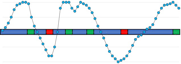
A vague summary of how a large portion of the genome might not actually be neutral. In this section of the genome, we have neutral (blue), maladaptive (red) and adaptive (green) elements. Natural selection either favours, disfavours, or is ambivalent about each of this sections alone. However, there is significant ‘spill-over’ around regions of positively or negatively selected sections, which causes the allele frequency of even the neutral sections to fluctuate widely. The blue dotted line represents this: when the line is above the genome, allele frequency is increased; when it is below it is decreased. As we travel along this section of the genome, you may notice it is rarely ever in the middle (the so-called ‘neutral‘ allele frequency, in line with the genome).
Although I avoid having a strong stance here (if you’re an evolutionary geneticist yourself, I will allow you to draw your own conclusions), it is my belief that the model of neutral theory – and the methods that rely upon it – are still fundamental to our understanding of evolution. Although it may present itself as a more conservative way to identify adaptation within the genome, and cannot account for the effect of the above processes, neutral theory undoubtedly presents itself as a direct and well-implemented strategy to understand adaptation and demography.
A recurring analytical method, both within The G-CAT and the broader ecological genetic literature, is based on coalescent theory. This is based on the mathematical notion that mutations within genes (leading to new alleles) can be traced backwards in time, to the point where the mutation initially occurred. Given that this is a retrospective, instead of describing these mutation moments as ‘divergence’ events (as would be typical for phylogenetics), these appear as moments where mutations come back together i.e. coalesce.
Before we can explore the multitude of applications of the coalescent, we need to understand the fundamental underlying model. The initial coalescent model was described in the 1980s, built upon by a number of different ecologists, geneticists and mathematicians. However, John Kingman is often attributed with the formation of the original coalescent model, and the Kingman’s coalescent is considered the most basic, primal form of the coalescent model.
From a mathematical perspective, the coalescent model is actually (relatively) simple. If we sampled a single gene from two different individuals (for simplicity’s sake, we’ll say they are haploid and only have one copy per gene), we can statistically measure the probability of these alleles merging back in time (coalescing) at any given generation. This is the same probability that the two samples share an ancestor (think of a much, much shorter version of sharing an evolutionary ancestor with a chimpanzee).
Normally, if we were trying to pick the parents of our two samples, the number of potential parents would be the size of the ancestral population (since any individual in the previous generation has equal probability of being their parent). But from a genetic perspective, this is based on the genetic (effective) population size (Ne), multiplied by 2 as each individual carries two copies per gene (one paternal and one maternal). Therefore, the number of potential parents is 2Ne.
A graph of the probability of a coalescent event (i.e. two alleles sharing an ancestor) in the immediatelypreceding generation (i.e. parents) relatively to the size of the population. As one might expect, with larger population sizes there is low chance of sharing an ancestor in the immediately prior generation, as the pool of ‘potential parents’ increases.
If we have an idealistic population, with large Ne, random mating and no natural selection on our alleles, the probability that their ancestor is in this immediate generation prior (i.e. share a parent) is 1/(2Ne). Inversely, the probability they don’t share a parent is 1 − 1/(2Ne). If we add a temporal component (i.e. number of generations), we can expand this to include the probability of how many generations it would take for our alleles to coalesce as (1 – (1/2Ne))t-1 x 1/2Ne.
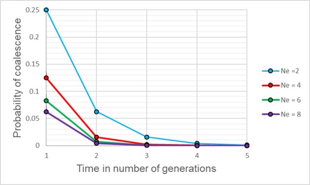
The probability of two alleles sharing a coalescent event back in time under different population sizes. Similar to above, there is a higher probability of an earlier coalescent event in smaller populations as the reduced number of ancestors means that alleles are more likely to ‘share’ an ancestor. However, over time this pattern consistently decreases under all population size scenarios.
Although this might seem mathematically complicated, the coalescent model provides us with a scenario of how we would expect different mutations to coalesce back in time if those idealistic scenarios are true. However, biology is rarely convenient and it’s unlikely that our study populations follow these patterns perfectly. By studying how our empirical data varies from the expectations, however, allows us to infer some interesting things about the history of populations and species.
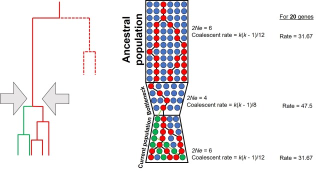
A diagram of how the coalescent can be used to detect bottlenecks in a single population (centre). In this example, we have contemporary population in which we are tracing the coalescence of two main alleles (red and green, respectively). Each circle represents a single individual (we are assuming only one allele per individual for simplicity, but for most animals there are up to two). Looking forward in time, you’ll notice that some red alleles go extinct just before the bottleneck: they are lost during the reduction in Ne. Because of this, if we measure the rate of coalescence (right), it is much higher during the bottleneck than before or after it. Another way this could be visualised is to generate gene trees for the alleles (left): populations that underwent a bottleneck will typically have many shorter branches and a long root, as many branches will be ‘lost’ by extinction (the dashed lines, which are not normally seen in a tree).
This makes sense from theoretical perspective as well, since strong genetic bottlenecks means that most alleles are lost. Thus, the alleles that we do have are much more likely to coalesce shortly after the bottleneck, with very few alleles that coalesce before the bottleneck event. These alleles are ones that have managed to survive the purge of the bottleneck, and are often few compared to the overarching patterns across the genome.
Testing migration (gene flow) across lineages
Another demographic factor we may wish to test is whether gene flow has occurred across our populations historically. Although there are plenty of allele frequency methods that can estimate contemporary gene flow (i.e. within a few generations), coalescent analyses can detect patterns of gene flow reaching further back in time.
A similar model of coalescence as above, but testing for migration rate (gene flow) in two recently diverged populations (right). In this example, when we trace two alleles (red and green) back in time, we notice that some individuals in Population 1 coalesce more recently with individuals of Population 2 than other individuals of Population 1 (e.g. for the red allele), and vice versa for the green allele. This can also be represented with gene trees (left), with dashed lines representing individuals from Population 2 and whole lines representing individuals from Population 1. This incomplete split between the two populations is the result of migration transferring genes from one population to the other after their initial divergence (also called ‘introgression’ or ‘horizontal gene transfer’).
Testing divergence time
In a similar vein, the coalescent can also be used to test how long ago the two contemporary populations diverged. Similar to gene flow, this is often included as an additional parameter on top of the coalescent model in terms of the number of generations ago. To convert this to a meaningful time estimate (e.g. in terms of thousands or millions of years ago), we need to include a mutation rate (the number of mutations per base pair of sequence per generation) and a generation time for the study species (how many years apart different generations are: for humans, we would typically say ~20-30 years).
An example of using the coalescent to test the divergence time between two populations, this time using three different alleles (red, green and yellow). Tracing back the coalescence of each alleles reveals different times (in terms of which generation the coalescence occurs in) depending on the allele (right). As above, we can look at this through gene trees (left), showing variation how far back the two populations (again indicated with bold and dashed lines respectively) split. The blue box indicates the range of times (i.e. a confidence interval) around which divergence occurred: with many more alleles, this can be more refined by using an ‘average’ and later related to time in years with a generation time.
While each of these individual concepts may seem (depending on how well you handle maths!) relatively simple, one critical issue is the interactive nature of the different factors. Gene flow, divergence time and population size changes will all simultaneously impact the distribution and frequency of alleles and thus the coalescent method. Because of this, we often use complex programs to employ the coalescent which tests and balances the relative contributions of each of these factors to some extent. Although the coalescent is a complex beast, improvements in the methodology and the programs that use it will continue to improve our ability to infer evolutionary history with coalescent theory.
Nugs are non-confrontational omnivorous species, preferring to hide and delve in the dark underground systems below the world of Thedas. Thus, nugs will typically avoid contact with people or predators by hiding in various crevices, using their pale skin to blend in with the surrounding rock faces. Reports of nugs in the wild demonstrate that nugs are remarkably inefficient at predator avoidance, despite their physiology; however, nug populations do not appear to suffer dramatically with predator presence, suggesting that either predators are too few to significantly impact population size or that alternative behaviours might allow them to rapidly bounce back from natural declines.
Given the lack of consistent light within their habitat, nugs are effectively blind, retaining only limited eyesight required for moving around above the surface. Nugs feed on a large variety of food sources, preferring insects but resorting to mineral deposits if available food resources are depleted. Their generalist diet may be one physiological trait that has allowed the nug to become some widespread and abundant historically.
Demography
Although the nug is a widespread and abundant species, they are heavily reliant on the connections of the Deep Roads to maintain connectivity and gene flow. With the gradual declination of Dwarven abundance and the loss of entire regions of the underground civilisation, it is likely that many areas of the nug distribution have become isolated and suffering from varying levels of inbreeding depression. Given the lack of access to these populations, whether some have collapsed since their isolation is unknown and potentially isolated populations may have even speciated if local environments have changed significantly.
Adaptive traits
Nugs are highly adapted to low-light, subterranean conditions, and show many phenotypic traits related to this kind of environment. The reduction of eyesight capability is considered a regression of unusable traits in underground habitats; instead, nugs show a highly developed and specialised nasal system. The high sensitivity of the nasal cavity makes them successful forages in the deep caverns of the underworld, and the elongated maw of the nug allows them to dig into buried food sources with ease. One of the more noticeable (and often disconcerting) traits of the nug is their human-like hands; the development of individual digits similar to fingers allows the nug to grip and manipulate rocky surfaces with surprising ease.
Management actions
Re-establishment of habitat corridors through the clearing and revival of the Deep Roads is critical for both reconnecting isolated populations of nugs and restoring natural gene flow, but also allowing access to remote populations for further studies. A combination of active removal of resident Darkspawn and population genetics analysis to accurately assess the conservation status of the species. That said, given the commercial value of the nug as a food source for many societies, establishing consistent sustainable farming practices may serve to both boost the nug populations and also provide an industry for many people.