In more fishy news, this week the latest (and last!) chapter of my PhD, describing how millions of years of climatic stability have allowed isolated and divergent lineages of pygmy perches to persist, was published (Open Access) in Heredity. It covers population divergence, phylogenetic relationships (including estimation of divergence times), species delimitation and projections of species distributions from the past (up to three million years ago) into the future (up to 2100). Some highlights include:
Continue readingFish
Fishy friends making the news
Bringing back the southern pygmy perch
You may recall (some months back), that I published a research paper describing the successful reintroduction of a threatened freshwater fish, the southern pygmy perch, into wetlands around Bendigo, Victoria. This work has been extremely rewarding for a lot of reasons: not just for the positive conservation outcomes for a threatened (and underappreciated!) species but also for the incredible community engagement it involved. Without the help of local volunteers, restoration efforts of this scale would not be possible and it’s been amazing to see how the community has responded. I really don’t think I can underestimate how invigorating it is to see the general public commit to direct conservation action and to be able to see the outcomes of their efforts over a few years.
Continue readingReviving rivers: a community-led tale of fish conservation
Communities and conservation
When I was younger, I used to love visiting our local creek: it was a beautiful spot of nature a short walk from home. On a couple occasions, my Dad took me to the creek to catch yabbies – for a suburban kid, it was one of the few times I actually held and interacted with wild biodiversity, and helped foster my love for conservation and inquiry into biology. In the late 2000s to early 2010s, a likely combination of local pollution and extensive drought extirpated the yabbies from the creek – I would never see one in that creek again. I was devastated for the local loss of a fascinating creature, and the connection to nature it represented, but felt powerless to remedy the situation. To my knowledge, there are still no yabbies in that creek.
Continue readingA tale of two fishes: how standing genetic diversity influences species responses to environmental change
How can species respond to environmental change?
If you’re a somewhat avid (or even cursory) reader of The G-CAT, you may remember my wrap-up post at the conclusion of my PhD in 2020 which described the various chapters of my thesis. Well, I’m pleased to announce that data chapter 2 of that thesis – on the comparative phylogeography of two threatened Australian freshwater fishes – has just been published in the journal BMC Ecology and Evolution. It’s a pretty complex paper which tackles genetic diversity, phylogenetics, demographic history, species distribution models and how these interact together to understand the evolutionary history of these species in a comparative framework. Feel free to check it out (it’s open access and free to read!) here.
Continue readingYou’re perfect, you’re beautiful, you look like a model (species)
What is a ‘model’?
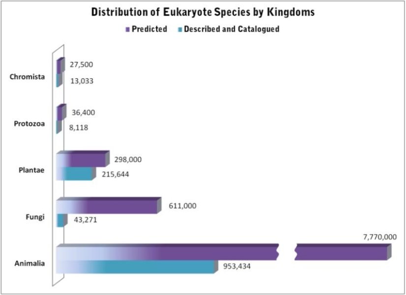
There are quite literally millions of species on Earth, ranging from the smallest of microbes to the largest of mammals. In fact, there are so many that we don’t actually have a good count on the sheer number of species and can only estimate it based on the species we actually know about. Unsurprisingly, then, the number of species vastly outweighs the number of people that research them, especially considering the sheer volumes of different aspects of species, evolution, conservation and their changes we could possibly study.
This is partly where the concept of a ‘model’ comes into it: it’s much easier to pick a particular species to study as a target, and use the information from it to apply to other scenarios. Most people would be familiar with the concept based on medical research: the ‘lab rat’ (or mouse). The common house mouse (Mus musculus) and the brown rat (Rattus norvegicus) are some of the most widely used models for understanding the impact of particular biochemical compounds on physiology and are often used as the testing phase of medical developments before human trials.
So, why are mice used as a ‘model’? What actually constitutes a ‘model’, rather than just a ‘relatively-well-research-species’? Well, there are a number of traits that might make certain species ideal subjects for understanding key concepts in evolution, biology, medicine and ecology. For example, mice are often used in medical research given their (relative) similar genetic, physiological and behavioural characteristics to humans. They’re also relatively short-lived and readily breed, making them ideal to observe the more long-term effects of medical drugs or intergenerational impacts. Other species used as models primarily in medicine include nematodes (Caenorhabditis elegans), pigs (Sus scrofa domesticus), and guinea pigs (Cavia porcellus).
The diversity of models
There are a wide variety and number of different model species, based on the type of research most relevant to them (and how well it can be applied to other species). Even with evolution and conservation-based research, which can often focus on more obscure or cryptic species, there are several key species that have widely been applied as models for our understanding of the evolutionary process. Let’s take a look at a few examples for evolution and conservation.
Drosophila
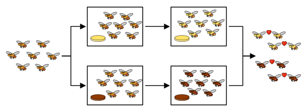
It would be remiss of me to not mention one of the most significant contributors to our understanding of the genetic underpinning of adaptation and speciation, the humble fruit fly (Drosophila melanogaster, among other species). The ability to rapidly produce new generations (with large numbers of offspring with very short generation time), small fully-sequenced genome, and physiological variation means that observing both phenotypic and genotypic changes over generations due to ‘natural’ (or ‘experimental’) selection are possible. In fact, Drosphilia spp. were key in demonstrating the formation of a new species under laboratory conditions, providing empirical evidence for the process of natural selection leading to speciation (despite some creationist claims that this has never happened).
Darwin’s finches
The original model of evolution could be argued to be Darwin’s finches, as the formed part of the empirical basis of Charles Darwin’s work on the theory of evolution by natural selection. This is because the different species demonstrate very distinct and obvious changes in morphology related to a particular diet (e.g. the physiological consequences of natural selection), spread across an archipelago in a clear demonstration of a natural experiment. Thus, they remain the original example of adaptive radiation and are fundamental components of the theory of evolution by natural selection. However, surprisingly, Darwin’s finches are somewhat overshadowed in modern research by other species in terms of the amount of available data.
Zebra finches
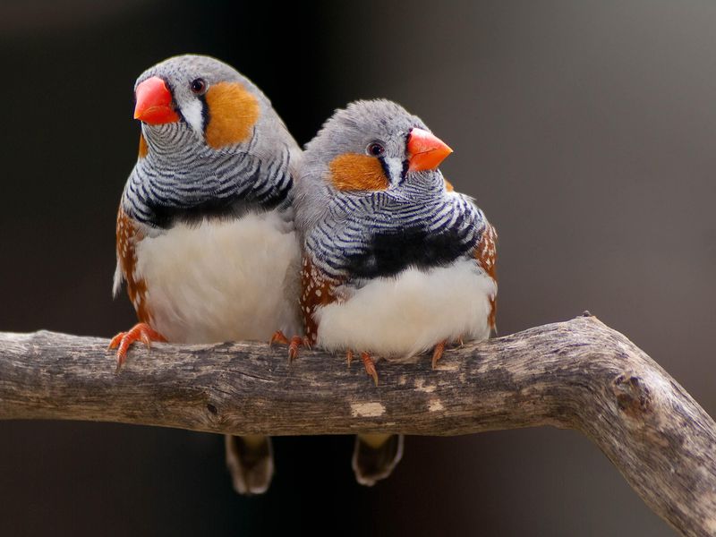
Even as far as birds go, one species clearly outshines the rest in terms of research. The zebra finch is one of the most highly researched vertebrate species, particularly as a model of song learning and behaviour in birds but also as a genetic model. The full genome of the zebra finch was the second bird to ever be sequenced (the first being a chicken), and remains one of the more detailed and annotated genomes in birds. Because of this, the zebra finch genome is often used as a reference for other studies on the genetics of bird species, especially when trying to understand the function of genetic changes or genes under selection.
Fishes
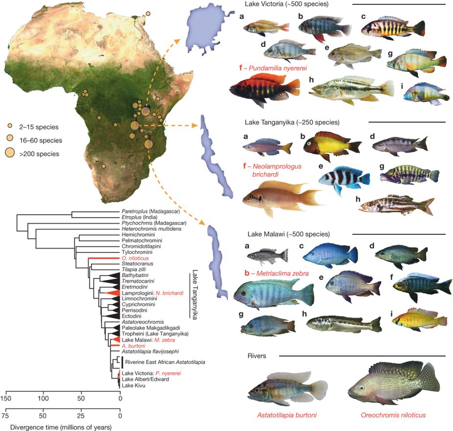
Fish are (perhaps surprisingly) also relatively well research in terms of evolutionary studies, largely due to their ancient origins and highly diverse nature, with many different species across the globe. They also often demonstrate very rapid and strong bouts of divergence, such as the cichlid fish species of African lakes which demonstrate how new species can rapidly form when introduced to new and variable environments. The cichlids have become the poster child of adaptive radiation in fishes much in the same way that Darwin’s finches highlighted this trend in birds. Another group of fish species used as a model for similar aspects of speciation, adaptive divergence and rapid evolutionary change are the three-spine and nine-spine stickleback species, which inhabit a variety of marine, estuarine and freshwater environments. Thus, studies on the genetic changes across these different morphotypes is a key in understanding how adaptation to new environments occur in nature (particularly the relatively common transition into different water types in fishes).
Zebra fish
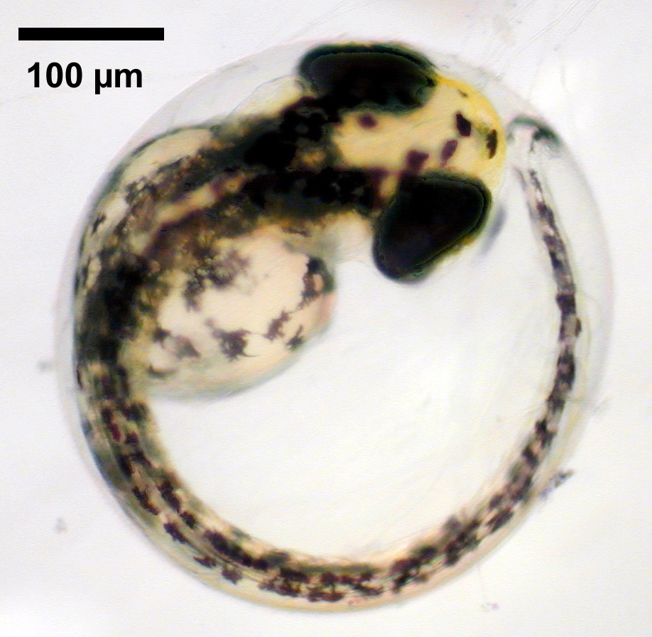
More similar to the medical context of lab rats is the zebrafish (ironically, zebra themselves are not considered a model species). Zebrafish are often used as models for understanding embryology and the development of the body in early formation given the rapid speed at which embryonic development occurs and the transparent body of embryos (which makes it easier to detect morphological changes during embryogenesis).
Using information from model species for non-models
While the relevance of information collected from model species to other non-model species depends on the similarity in traits of the two species, our understanding of broad concepts such as evolutionary process, biochemical pathways and physiological developments have significantly improved due to model species. Applying theories and concepts from better understood organisms to less researched ones allows us to produce better research much faster by cutting out some of the initial investigative work on the underlying processes. Thus, model species remain fundamental to medical advancement and evolutionary theory.
That said, in an ideal world all species would have the same level of research and resources as our model species. In this sense, we must continue to strive to understand and research the diversity of life on Earth, to better understand the world in which we live. Full genomes are progressively being sequenced for more and more species, and there are a number of excellent projects that are aiming to sequence at least one genome for all species of different taxonomic groups (e.g. birds, bats, fish). As the data improves for our non-model species, our understanding of evolution, conservation management and medical research will similarly improve.
