This is the fourth (and final) part of the miniseries on the genetics and process of speciation. To start from Part One, click here.
In last week’s post, we looked at how we can use genetic tools to understand and study the process of speciation, and particularly the transition from populations to species along the speciation continuum. Following on from that, the question of “how many species do I have?” can be further examined using genetic data. Sometimes, it’s entirely necessary to look at this question using genetics (and genomics).
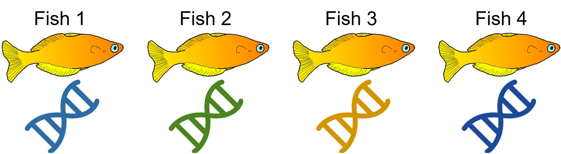
An example of cryptic species. All four fish in this figure are morphologically identical to one another, but they differ in their underlying genetic variation (indicated by the different colours of DNA). Thus, from looking at these fish alone we would not perceive any differences, but their genetic make-up might suggest that there are more than one species…
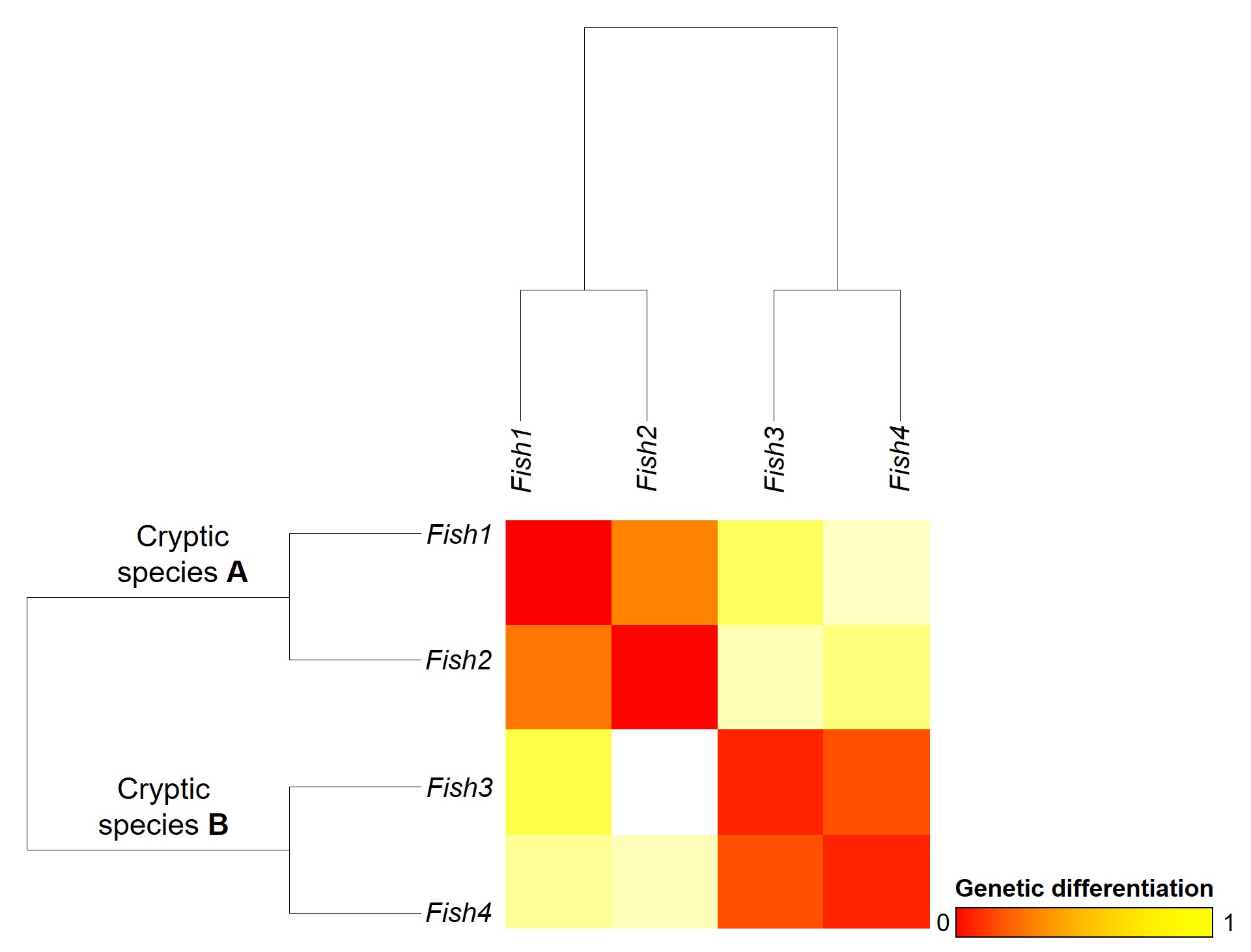
The level of genetic differentiation between the fish in the above example. The phylogenies on the left and top of the figure demonstrate the evolutionary relationships of these four fish. The matrix shows a heatmap of the level of differences between different pairwise comparisons of all four fish: red squares indicate zero genetic differences (such as when comparing a fish to itself; the middle diagonal) whilst yellow squares indicate increasingly higher levels of genetic differentiation (with bright yellow = all differences). By comparing the different fish together, we can see that Fish 1 and 2, and Fish 3 and 4, are relatively genetically similar to one another (red-deep orange). However, other comparisons show high level of genetic differences (e.g. 1 vs 3 and 1 vs 4). Based on this information, we might suggest that Fish 1 and 2 belong to one cryptic species (A) and Fish 3 and 4 belong to a second cryptic species (B).
Genetic tools to study species: the ‘Barcode of Life’
A classically employed method that uses DNA to detect and determine species is referred to as the ‘Barcode of Life’. This uses a very specific fragment of DNA from the mitochondria of the cell: the cytochrome c oxidase I gene, CO1. This gene is made of 648 base pairs and is found pretty well universally: this and the fact that CO1 evolves very slowly make it an ideal candidate for easily testing the identity of new species. Additionally, mitochondrial DNA tends to be a bit more resilient than its nuclear counterpart; thus, small or degraded tissue samples can still be sequenced for CO1, making it amenable to wildlife forensics cases. Generally, two sequences will be considered as belonging to different species if they are certain percentage different from one another.
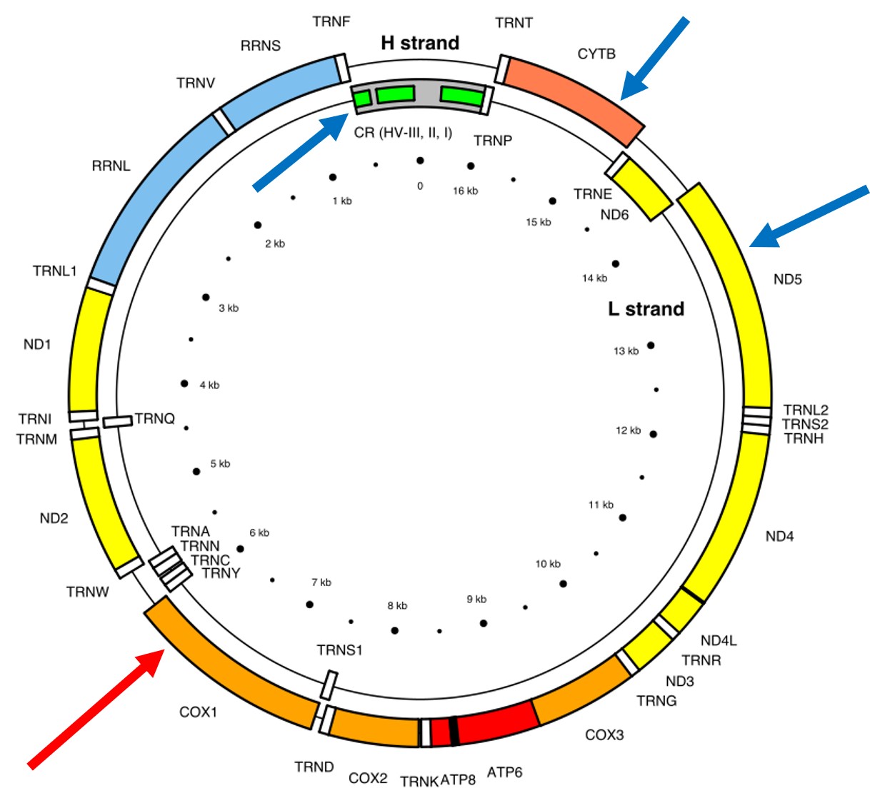
The full (annotated) mitochondrial genome of humans, with the different genes within it labelled. The CO1 gene is labelled with the red arrow (sometimes also referred to as COX1) whilst blue arrows point to other genes often used in phylogenetic or taxonomic studies, depending on the group or species in question.
Despite the apparent benefits of CO1, there are of course a few drawbacks. Most of these revolve around the mitochondrial genome itself. Because mitochondria are passed on from mother to offspring (and not at all from the father), it reflects the genetic history of only one sex of the species. Secondly, the actual cut-off for species using CO1 barcoding is highly contentious and possibly not as universal as previously suggested. Levels of sequence divergence of CO1 between species that have been previously determined to be separate (through other means) have varied from anywhere between 2% to 12%. The actual translation of CO1 sequence divergence and species identity is not all that clear.
Gene tree – species tree incongruences
One particularly confounding aspect of defining species based on a single gene, and with using phylogenetic-based methods, is that the history of that gene might not actually be reflective of the history of the species. This can be a little confusing to think about but essentially leads to what we call “gene tree – species tree incongruence”. Different evolutionary events cause different effects on the underlying genetic diversity of a species (or group of species): while these may be predictable from the genetic sequence, different parts of the genome might not be as equally affected by the same exact process.
A classic example of this is hybridisation. If we have two initial species, which then hybridise with one another, we expect our resultant hybrids to be approximately made of 50% Species A DNA and 50% Species B DNA (if this is the first generation of hybrids formed; it gets a little more complicated further down the track). This means that, within the DNA sequence of the hybrid, 50% of it will reflect the history of Species A and the other 50% will reflect the history of Species B, which could differ dramatically. If we randomly sample a single gene in the hybrid, we will have no idea if that gene belongs to the genealogy of Species A or Species B, and thus we might make incorrect inferences about the history of the hybrid species.
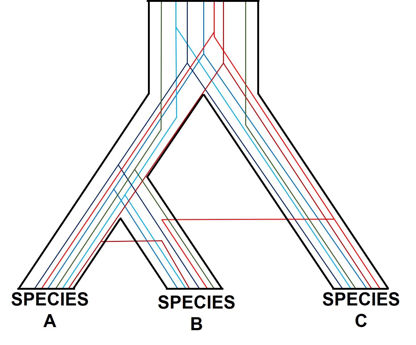
A diagram of gene tree – species tree incongruence. Each individual coloured line represents a single gene as we trace it back through time; these are mostly bound within the limits of species divergences (the black borders). For many genes (such as the blue ones), the genes resemble the pattern of species divergences very well, albeit with some minor differences in how long ago the splits happened (at the top of the branches). However, the red genes contrast with this pattern, with clear movement across species (from A and C into B): this represents genes that have been transferred by hybridisation. The green line represents a gene affected by what we call incomplete lineage sorting; that is, we cannot trace it back far enough to determine exactly how/when it initially diverged and so there are still two separate green lines at the very top of the figure. You can think of each line as a separate phylogenetic tree, with the overarching species tree as the average pattern of all of the genes.
There are a number of other processes that could similarly alter our interpretations of evolutionary history based on analysing the genetic make-up of the species. The best way to handle this is simply to sample more genes: this way, the effect of variation of evolutionary history in individual genes is likely to be overpowered by the average over the entire gene pool. We interpret this as a set of individual gene trees contained within a species tree: although one gene might vary from another, the overall picture is clearer when considering all genes together.
Species delimitation
In earlier posts on The G-CAT, I’ve discussed the biogeographical patterns unveiled by my Honours research. Another key component of that paper involved using statistical modelling to determine whether cryptic species were present within the pygmy perches. I didn’t exactly elaborate on that in that section (mostly for simplicity), but this type of analysis is referred to as ‘species delimitation’. To try and simplify complicated analyses, species delimitation methods evaluate possible numbers and combinations of species within a particular dataset and provides a statistical value for which configuration of species is most supported. One program that employs species delimitation is Bayesian Phylogenetics and Phylogeography(BPP): to do this, it uses a plethora of information from the genetics of the individuals within the dataset. These include how long ago the different populations/species separated; which populations/species are most related to one another; and a pre-set minimum number of species (BPP will try to combine these in estimations, but not split them due to computational restraints). This all sounds very complex (and to a degree it is), but this allows the program to give you a statistical value for what is a species and what isn’t based on the genetics and statistical modelling.
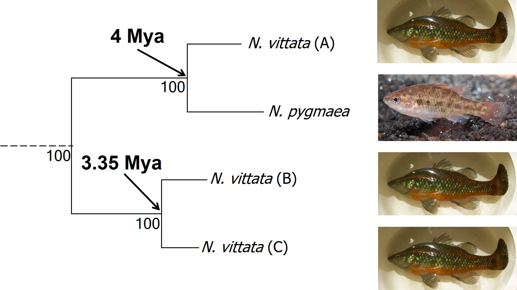
The cryptic species of pygmy perches identified within my research paper. This represents part of the main phylogenetic tree result, with the estimates of divergence times from other analyses included. The pictures indicate the physiology of the different ‘species’: Nannoperca pygmaea is morphologically different to the other species of Nannoperca vittata. Species delimitation analysis suggested all four of these were genetically independent species; at the very least, it is clear that there must be at least 2 species of Nannoperca vittata since A is more related to N. pygmaea than to other N. vittata species. Photo credits: N. vittata = Chris Lamin; N. pygmaea = David Morgan.
The end result of a BPP run is usually reported as a species tree (e.g. a phylogenetic tree describing species relationships) and statistical support for the delimitation of species (0-1 for each species). Because of the way the statistical component of BPP works, it has been found to give extremely high support for species identities. This has been criticised as BPP can, at time, provide high statistical support for genetically isolated lineages (i.e. divergent populations) which are not actually species.
Improving species identities with integrative taxonomy
Due to this particular drawback, and the often complex nature of species identity, using solely genetic information such as species delimitation to define species is extremely rare. Instead, we use a combination of different analytical techniques which can include genetic-based evaluations to more robustly assign and describe species. In my own paper example, we suggested that up to three ‘species’ of N. vittata that were determined as cryptic species by BPP could potentially exist pending on further analyses. We did not describe or name any of the species, as this would require a deeper delve into the exact nature and identity of these species.
As genetic data and analytical techniques improve into the future, it seems likely that our ability to detect and determine species boundaries will also improve. However, the additional supported provided by alternative aspects such as ecology, behaviour and morphology will undoubtedly be useful in the progress of taxonomy.
Given the strong influence of genetic identity on the process and outcomes of the speciation process, it seems a natural connection to use genetic information to study speciation and species identities. There is a plethora of genetics-based tools we can use to investigate how speciation occurs (both the evolutionary processes and the external influences that drive it). One clear way to test whether two populations of a particular species are actually two different species is to investigate genes related to reproductive isolation: if the genetic differences demonstrate reproductive incompatibilities across the two populations, then there is strong evidence that they are separate species (at least under the Biological Species Concept; see Part One for why!). But this type of analysis requires several tools: 1) knowledge of the specific genes related to reproduction (e.g. formation of sperm and eggs, genital morphology, etc.), 2) the complete and annotated genome of the species (to be able to find and analyse the right genes properly) and 3) a good amount of data for the populations in question. As you can imagine, for people working on non-model species (i.e. ones that haven’t had the same history and detail of research as, say, humans and mice), this can be problematic. So, instead, we can use other genetic information to investigate and suggest patterns and processes related to the formation of new species.
Is reproductive isolation naturally selected for or just a consequence?
A fundamental aspect of studies of speciation is a “chicken or the egg”-type paradigm: does natural selection directly select for rapid reproductive isolation, preventing interbreeding; or as a secondary consequence of general adaptive differences, over a long history of evolution? This might be a confusing distinction, so we’ll dive into it a little more.
Of the two proposed models of speciation, the by-product of natural selection (the second model) has been the more favoured. Simply put, this expands on Darwin’s theory of evolution that describes two populations of a single species evolving independently of one another. As these become more and more different, both in physical (‘phenotype’) and genetic (‘genotype’) characteristics, there comes a turning point where they are so different that an individual from one population could not reasonably breed with an individual from the other to form a fertile offspring. This could be due to genetic incompatibilities (such as different chromosome numbers), physiological differences (such as changes in genital morphology), or behavioural conflicts (such as solitary vs. group living).
Certainly, this process makes sense, although it is debatable how fast reproductive isolation would occur in a given species (or whether it is predictable just based on the level of differentiation between two populations). Another model suggests that reproductive isolation actually might arise very quickly if natural selection favours maintaining particular combinations of traits together. This can happen if hybrids between two populations are not particularly well adapted (fit), causing natural selection to favour populations to breed within each group rather than across groups (leading to reproductive isolation). Typically, this is referred to as ‘reinforcement’ and predominantly involves isolating mechanisms that prevent individuals across populations from breeding in the first place (since this would be wasted energy and resources producing unfit offspring). The main difference between these two models is the sequence of events: do populations ecologically diverge, and because of that then become reproductively isolated, or do populations selectively breed (enforcing reproductive isolation) and thus then evolve independently?
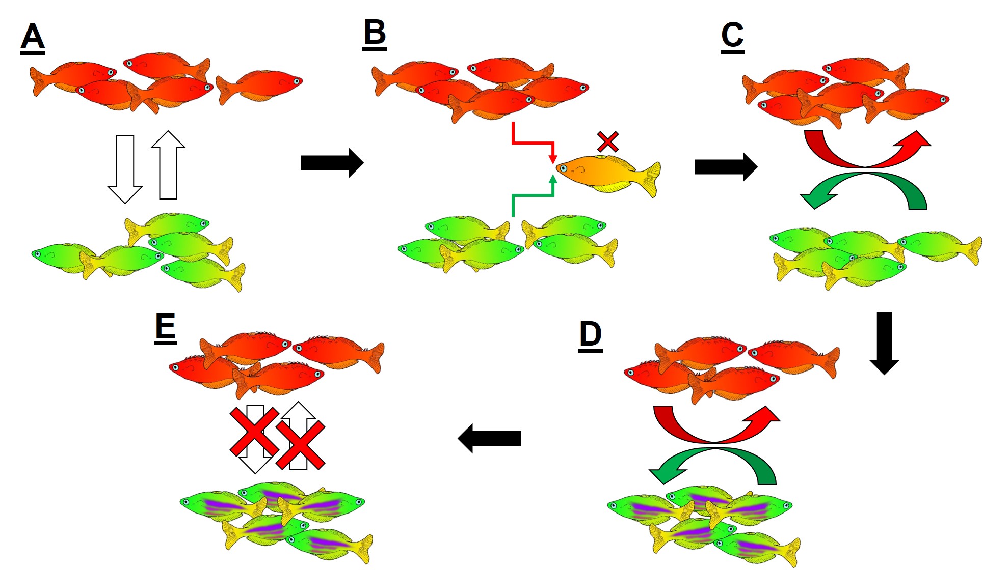
An example of reinforcement leading to speciation. A) We start with two populations of a single species (a red fish population and a green fish population), which can interbreed (the arrows). B) Because these two groups can breed, hybrids of the two populations can be formed. However, due to the poor combination of red and green fish genes within a hybrid, they are not overly fit (the red cross). C) Since natural selection doesn’t favour forming hybrids, populations then adapt to selectively breed only with similar fish, reducing the amount of interbreeding that occurs. D) With the two populations effectively isolated from one another, different adaptations specific to each population (spines in red fish, purple stripes in green fish) can evolve, causing them to further differentiate. E) At some point in the differentiation process, hybrids move from being just selectively unfit (as in B)) to entirely impossible, thus making the two populations formal species. In this example, evolution has directly selected against hybrids first, thus then allowing ecological differences to occur (as opposed to the other way around).
Reproductive isolation through DMIs
The reproductive incompatibility of two populations (thus making them species) is often intrinsically linked to the genetic make-up of those two species. Some conflicts in the genetics of Population 1 and Population 2 may mean that a hybrid having half Population 1 genes and half Population 2 genes will have serious fitness problems (such as sterility or developmental problems). Dramatic genetic differences, particularly a difference in the number of chromosomes between the two sources, is a significant component of reproductive isolation and is usually to blame for sterile hybrids such as ligers, zorse and mules.
However, subtler genetic differences can also have a strong effect: for example, the unique combination of Population 1 and Population 2 genes within a hybrid might interact with one another negatively and cause serious detrimental effects. These are referred to as “Dobzhansky-Müller Incompatibilities” (DMIs) and are expected to accumulate as the two populations become more genetically differentiated from one another. This can be a little complicated to imagine (and is based upon mathematical models), but the basis of the concept is that some combinations of gene variants have never, over evolutionary history, been tested together as the two populations diverge. Hybridisation of these two populations suddenly makes brand new combinations of genes, some of which may be have profound physiological impacts (including on reproduction).
An example of how Dobzhansky-Müller Incompatibilities arise, adapted from Coyne & Orr (2004). We start with an initial population (center top), which splits into two separate populations. In this example, we’ll look at how 5 genes (each letter = one gene) change over time in the separate populations, with the original allele of the gene (lowercase) occasionally mutating into a new allele (upper case). These mutations happen at random times and in random genes in each population (the red letters), such that the two become very different over time. After a while, these two populations might form hybrids; however, given the number of changes in each population, this hybrid might have some combinations of alleles that are ‘untested’ in their evolutionary history (see below). These untested combinations may cause the hybrid to be infertile or unviable, making the two populations isolated species.
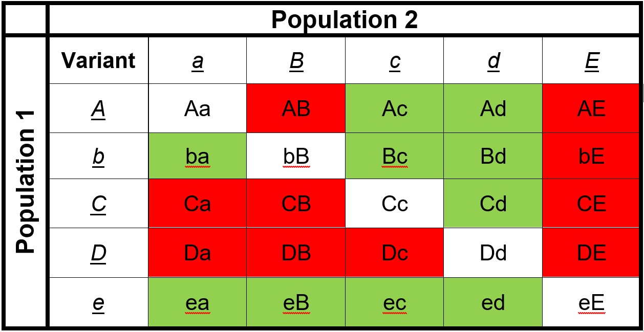
The list of ‘untested’ genetic combinations from the above example. This table shows the different combinations of each gene that could be made in a hybrid if these two populations interbred. The red cells indicate combinations that have never been ‘tested’ together; that is, at no point in the evolutionary history of these two populations were those two particular alleles together in the same individual. Green cells indicate ones that were together at some point, and thus are expected to be viable combinations (since the resultant populations are obviously alive and breeding).
How can we look at speciation in action?
We can study the process of speciation in the natural world without focussing on the ‘reproductive isolation’ element of species identity as well. For many species, we are unlikely to have the detail (such as an annotated genome and known functions of genes related to reproduction) required to study speciation at this level in any case. Instead, we might choose to focus on the different factors that are currently influencing the process of speciation, such as how the environmental, demographic or adaptive contexts of populations plays a role in the formation of new species. Many of these questions fall within the domain of phylogeography; particularly, how the historical environment has shaped the diversity of populations and species today.
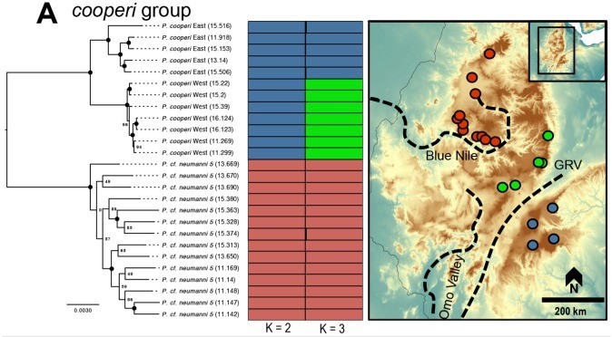
An example of the interplay between speciation and phylogeography, taken from Reyes-Velasco et al. (2018). They investigated the phylogeographic history of several different groups of species within the frog genus Ptychadena; in this figure, we can see how the different species (indicated by the colours and tree on the left) relate to the geography of their habitat (right).
A variety of different analytical techniques can be used to build a picture of the speciation process for closely related or incipient species. A good starting point for any speciation study is to look at how the different study populations are adapting; is there evidence that natural selection is pushing these populations towards different genotypes or ecological niches? If so, then this might be a precursor for speciation, and we can build on this inference with other complementary analyses.
For example, estimating divergence times between populations can help us suggest whether there has been sufficient time for speciation to occur (although this isn’t always clear cut). Additionally, we could estimate the levels of genetic hybridisation (‘introgression’) between two populations to suggest whether they are reasonably isolated and divergent enough to be considered functional species.
The future of speciation genomics
Although these can help answer some questions related to speciation, new tools are constantly needed to provide a clearer picture of the process. Understanding how and why new species are formed is a critical aspect of understanding the world’s biodiversity. How can we predict if a population will speciate at some point? What environmental factors are most important for driving the formation of new species? How stable are species identities, really? These questions (and many more) remain elusive for a wide variety of life on Earth.
This is Part 1 of a four part miniseries on the process of speciation; how we get new species, how we can see this in action, and the end results of the process. This week, we’ll start with a seemingly obvious question: what is a species?
The definition of a ‘species’
‘Species’ are a human definition of the diversity of life. When we talk about the diversity of life, and the myriad of creatures and plants on Earth, we often talk about species diversity. This might seem glaringly obvious, but there’s one key issue: what is a species, anyway? While we might like to think of them as discrete and obvious groups (a dog is definitely not the same species as a cat, for example), the concept of a singular “species” is actually the result of human categorisation.
In reality, the diversity of life is spread across a huge spectrum of differentiation: from things which are closely related but still different to us (like chimps), to more different again (other mammals), to hardly relatable at all (bacteria and plants). So, what is the cut-off for calling something a species, and not a different genus, family, or kingdom? Or alternatively, at what point do we call a specific sub-group of a species as a sub-species, or another species entirely?
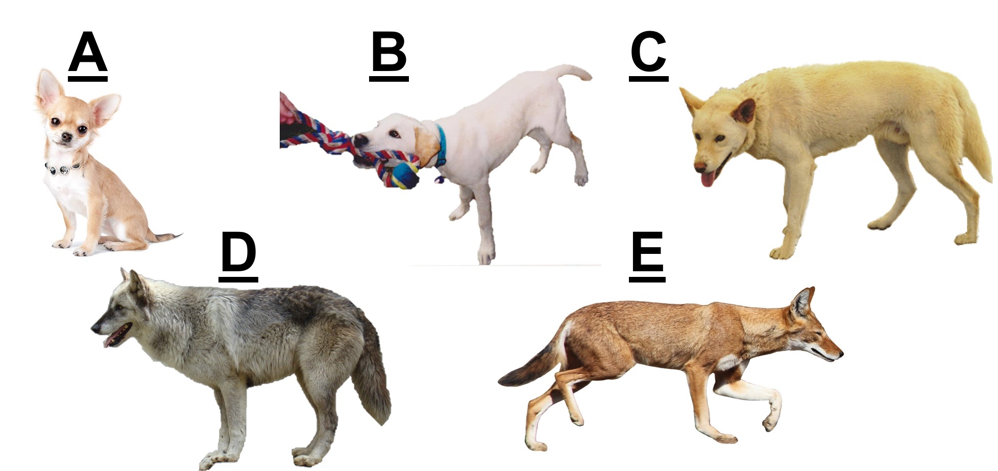
This might seem like a simple question: we look at two things, and they look different, so they must be different species, right? Well, of course, nature is never simple, and the line between “different” and “not different” is very blurry. Here’s an example: consider that you knew nothing about the history, behaviour or genetics of dogs. If you simply looked at all the different breeds of dogs on Earth, you might suggest that there are hundreds of species of domestic dogs. That seems a little excessive though, right? In fact, the domestic dog, Eurasian wolf, and the Australian dingo are all the same species (but different subspecies, along with about 38 others…but that’s another issue altogether).
Morphology can be misleading for identifying species. In this example, we have A) a dog, B) also a dog, C) still a dog, D) yet another dog, and E) not a dog. For the record, A-D are all Canis lupus of some variety; A and B are domestic dogs (Canis lupus familiaris), C is a dingo (Canis lupus dingo) and D is a grey wolf (Canis lupus lupus). E, however, isthe Ethiopian wolf, Canis simensis.
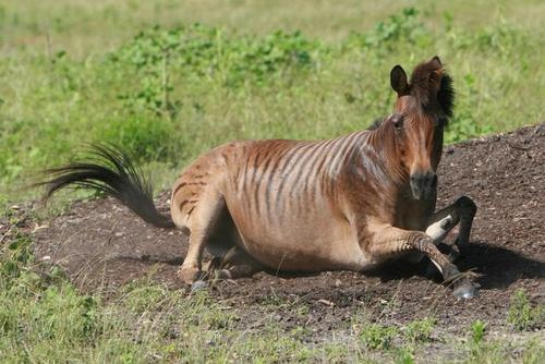
For example, a horse and zebra can breed to produce a zorse, however zorse are fundamentally infertile (due to the different number of chromosomes between a horse and a zebra) and thus a horse is a different species to a zebra. However, a German Shepherd and a chihuahua can breed and make a hybrid mutt, so they are the same species.
A zorse, which shows its hybrid nature through zebra stripes and horse colouring. These two are still separate species since zorses are infertile, and thus are not a singular stable entity.
An example of how reproductive isolation maintains genetic and evolutionary independence of species. In A), our cat groups are robust species, reproductively isolated from one another (as shown by the black box). When each species undergoes natural selection and their genetic variation changes (colour changes on the cats and DNA), these changes are kept within each lineage. This contrasts to B), where genetic changes can be transferred between species. Without reproductive isolation, evolution in the orange lineage and the blue lineage can combine within hybrids, sharing the evolutionary pathways of both ancestral species.
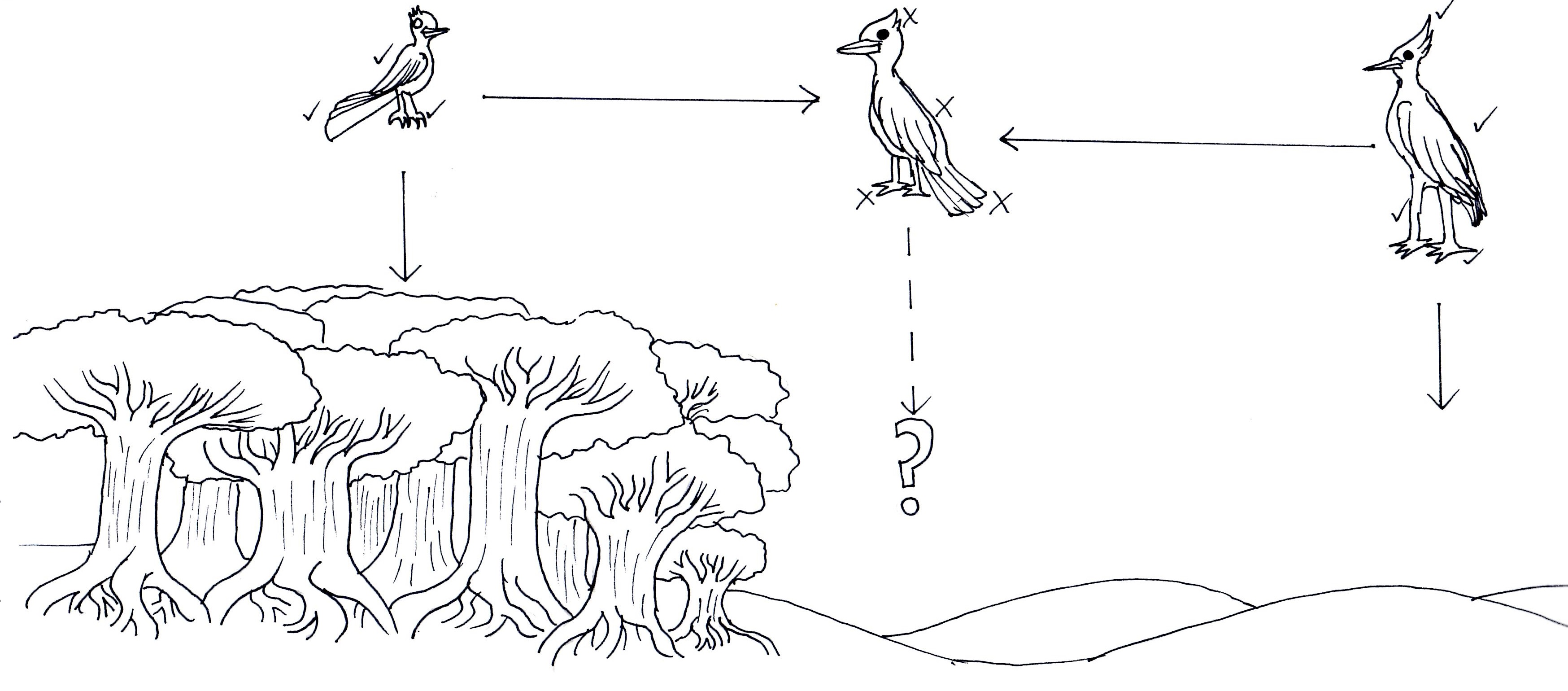
An example of unfit hybrids causing effective reproductive isolation. In this example, we have two different bird species adapted to very different habitats; a smaller, long-tailed bird (left) adapted to moving through dense forest, and a large, longer-legged bird (right) adapted to traversing arid deserts. When (or if) these two species hybridised, the resultant offspring would be middle of the road, possessing too few traits to be adaptive in either the forest or the desert and no fitting intermediate environment available. Measuring exactly how unfit this hybrid would be is a difficult task in establishing species boundaries.
Integrative taxonomy
To try and account for the issues with the BSC, taxonomists try to push for the usage of “integrative taxonomy”. This means that species should be defined by multiple different agreeing concepts, such as reproductive isolation, genetic differentiation, behavioural differences, and/or ecological traits. The more traits that can separate the two, the greater support there is for the species to be separated: if they disagree, then more information is needed to determine exactly whether or not that should be called different species. Debates about taxonomy are ongoing and are likely going to be relevant for years to come, but form critical components of understanding biodiversity, patterns of evolution, and creating effective conservation legislation to protect endangered or threatened species (for whichever groups we decide are species).
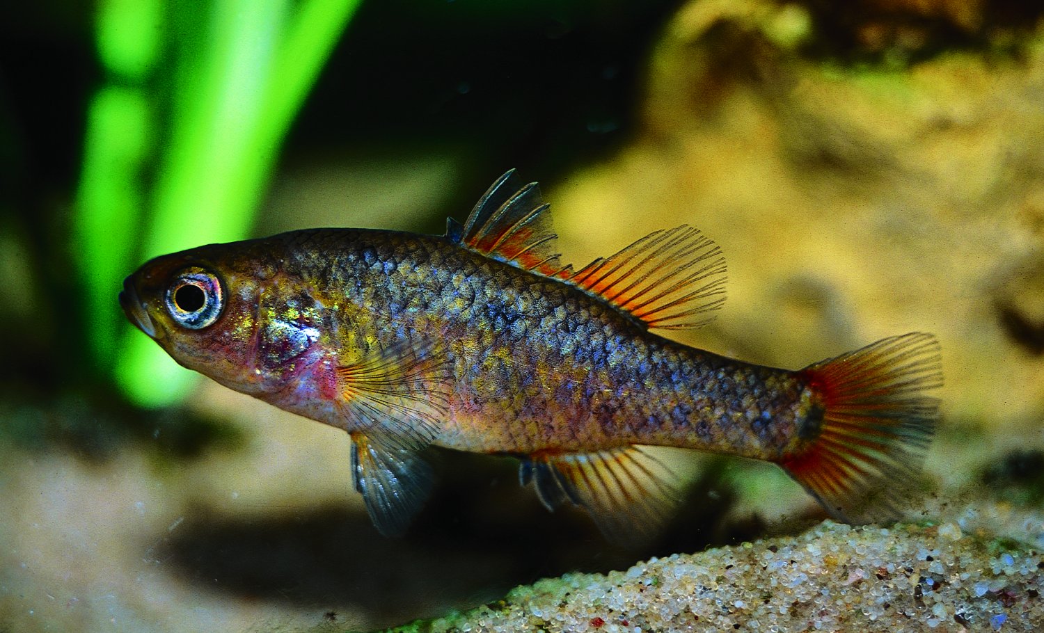
As regular readers of The G-CAT are likely aware, my first ever scientific paper was published this week. The paper is largely the results of my Honours research (with some extra analysis tacked on) on the phylogenomics (the same as phylogenetics, but with genomic data) and biogeographic history of a group of small, endemic freshwater fishes known as the pygmy perch. There are a number of different messages in the paper related to biogeography, taxonomy and conservation, and I am really quite proud of the work.
A male southern pygmy perch, which usually measures 6-8 cm long.
To my honest surprise, the paper has received a decentamount of media attention following its release. Nearly all of these have focused on the biogeographic results and interpretations of the paper, which is arguably the largest component of the paper. In these media releases, the articles are often opened with “…despite the odds, new research has shown how a tiny fish managed to find its way across the arid Australian continent – more than once.” So how did they manage it? These are tiny fish, and there’s a very large desert area right in the middle of Australia, so how did they make it all the way across? And more than once?!
The Great (southern) Southern Land
To understand the results, we first have to take a look at the context for the research question. There are seven officially named species of pygmy perches (‘named’ is an important characteristic here…but we’ll go into the details of that in another post), which are found in the temperate parts of Australia. Of these, three are found with southwest Western Australia, in Australia’s only globally recognised biodiversity hotspot, and the remaining four are found throughout eastern Australia (ranging from eastern South Australia to Tasmania and up to lower Queensland). These two regions are separated by arid desert regions, including the large expanse of the Nullarbor Plain.
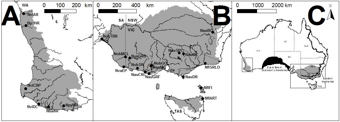
The distributions of pygmy perch species across Australia. The dots and labels refer to different sampling sites used in the study. A: the distribution of western pygmy perches, and essentially the extent of the southwest WA biodiversity hotspot region. B: the distribution of eastern pygmy perches, excluding N. oxleyana which occurs in upper NSW/lower QLD (indicated in C). C: the distributions relative to the map of Australia. The black region in the middle indicates the Nullarbor Plain.
The Nullarbor Plain is a remarkable place. It’s dead flat, has no trees, and most importantly for pygmy perches, it also has no standing water or rivers. The plain was formed from a large limestone block that was pushed up from beneath the Earth approximately 15 million years ago; with the progressive aridification of the continent, this region rapidly lost any standing water drainages that would have connected the east to the west. The remains of water systems from before (dubbed ‘paleodrainages’) can be seen below the surface.
See? Nothing here. Photo taken near Watson, South Australia. Credit: Benjamin Rimmer.
Biogeography of southern Australia
As one might expect, the formation of the Nullarbor Plain was a huge barrier for many species, especially those that depend on regular accessible water for survival. In many species of both plants and animals, we see in their phylogenetic history a clear separation of eastern and western groups around this time; once widely distributed species become fragmented by the plain and diverged from one another. We would most certainly expect this to be true of pygmy perch.
But our questions focus on what happened before the Nullarbor Plain arrived in the picture. More than 15 million years ago, southern Australia was a massively different place. The climate was much colder and wetter, even in central Australia, and we even have records of tropical rainforest habitats spreading all the way down to Victoria. Water-dependent animals would have been able to cross the southern part of the continent relatively freely.
Biogeography of the enigmatic pygmy perches
This is where the real difference between everything else and pygmy perch happens. For most species, we see only one east and west split in their phylogenetic tree, associated with the Nullarbor Plain; before that, their ancestors were likely distributed across the entire southern continent and were one continuous unit.
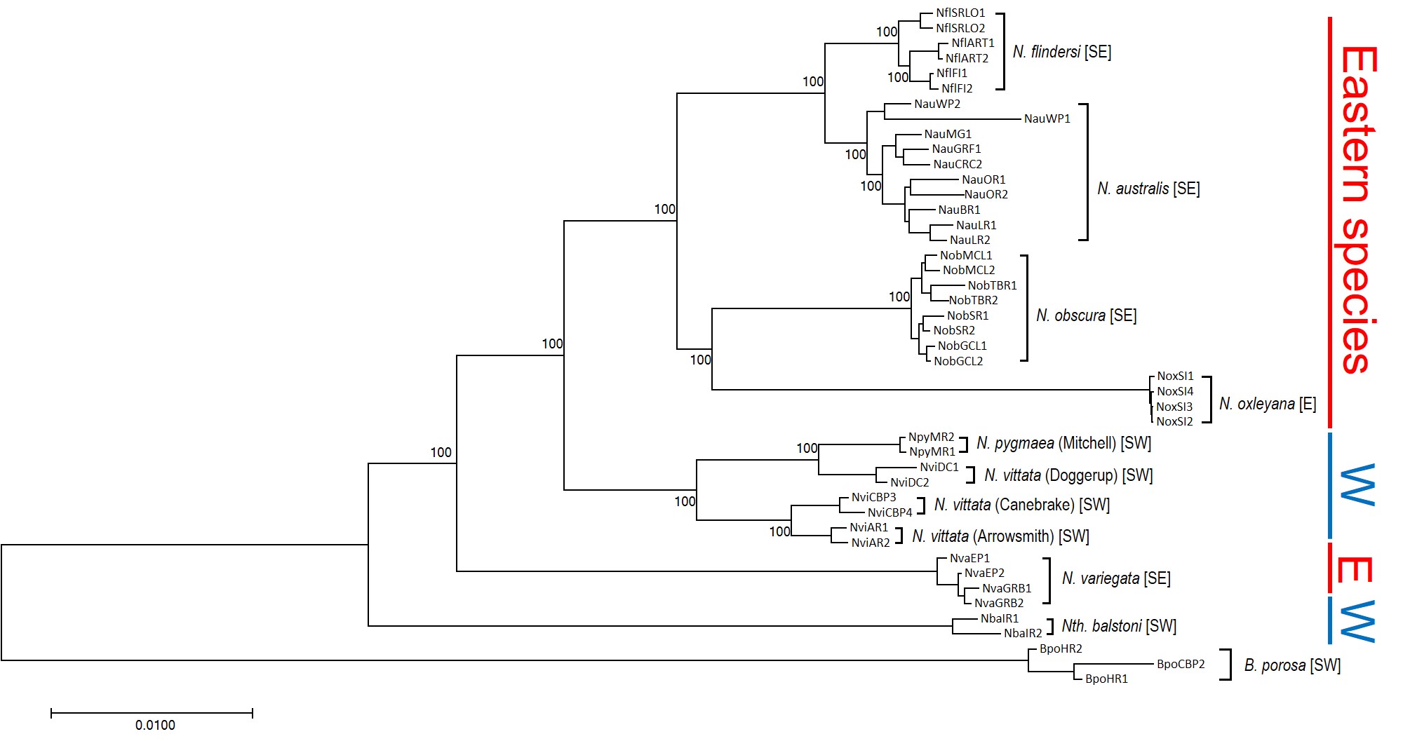
Not for pygmy perch, though. Our phylogenetic patterns show that there were multiple splits between eastern and western ancestral pygmy perch. We can see this visually within the phylogenetic tree; some western species of pygmy perches are more closely related, from an evolutionary perspective, to eastern species of pygmy perches than they are to other western species. This could imply a couple different things; either some species came about by migration from east to west (or vice versa), and that this happened at least twice, or that two different ancestral pygmy perches were distributed across all of southern Australia and each split east-west at some point in time. These two hypotheses are called “multiple invasion” and “geographic paralogy”, respectively.
The phylogeny of pygmy perches produced by this study, containing 45 different individuals across all species of pygmy perch. Species are labelled in the tree in brackets, and their geographic location (east or west) is denoted by the colour on the right. This tree clearly shows more than one E/W separation, as not all eastern species are within the same clade. For example, despite being an eastern species, N. variegata is more closely related to Nth. balstoni or N. vittata than to the other eastern species (N. australis, N. obscura, N. oxleyana and N. ‘flindersi’.
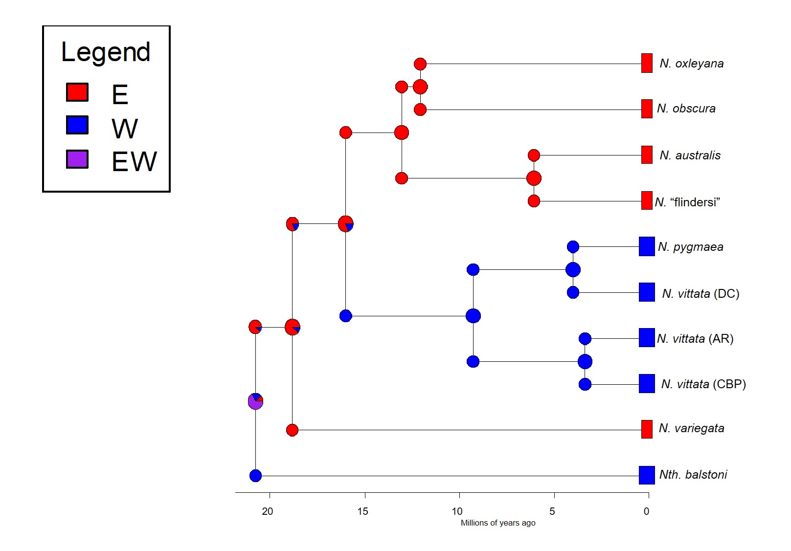
So, which is it? We delved deeper into this using a type of analysis called ‘ancestral clade reconstruction’. This tries to guess the likely distributions of species ancestors using different models and statistical analysis. Our results found that the earliest east-west split was due to the fragmentation of a widespread ancestor ~20 million years ago, and a migration event facilitated by changing waterways from the Nullarbor Plain pushing some eastern pygmy perches to the west to form the second group of western species. We argue for more than one migration across Australia since the initial ancestor of pygmy perches must have expanded from some point (either east or west) to encompass the entirety of southern Australia.
The ancestral area reconstruction of pygmy perches, estimated using the R package BioGeoBEARS. The different pie charts denote the relative probability of the possible distributions for the species or ancestor at that particular time; colours denote exactly where the distribution is (following the legend). As you can see, the oldest E/W split at 21 million years ago likely resulted from a single widespread ancestor, with it’s range split into an east and west group. The second E/W event, at 15 million years ago, most likely reflects a migration from east to west, resulting in the formation of the N. vittata species group. This coincides with the Nullarbor Plain, so it’s likely that changes in waterway patterns allowed some eastern pygmy perch to move westward as the area became more arid.
So why do we see this for pygmy perch and no other species? Well, that’s the real mystery; out of all of the aquatic species found in southeast and southwest Australia, pygmy perch are one of the worst at migrating. They’re very picky about habitat, small, and don’t often migrate far unless pushed (by, say, a flood). It is possible that unrecorded extinct species of pygmy perch might help to clarify this a little, but the chances of finding a preserved fish fossil (let alone for a fish less than 8cm in size!) is extremely unlikely. We can really only theorise about how they managed to migrate.
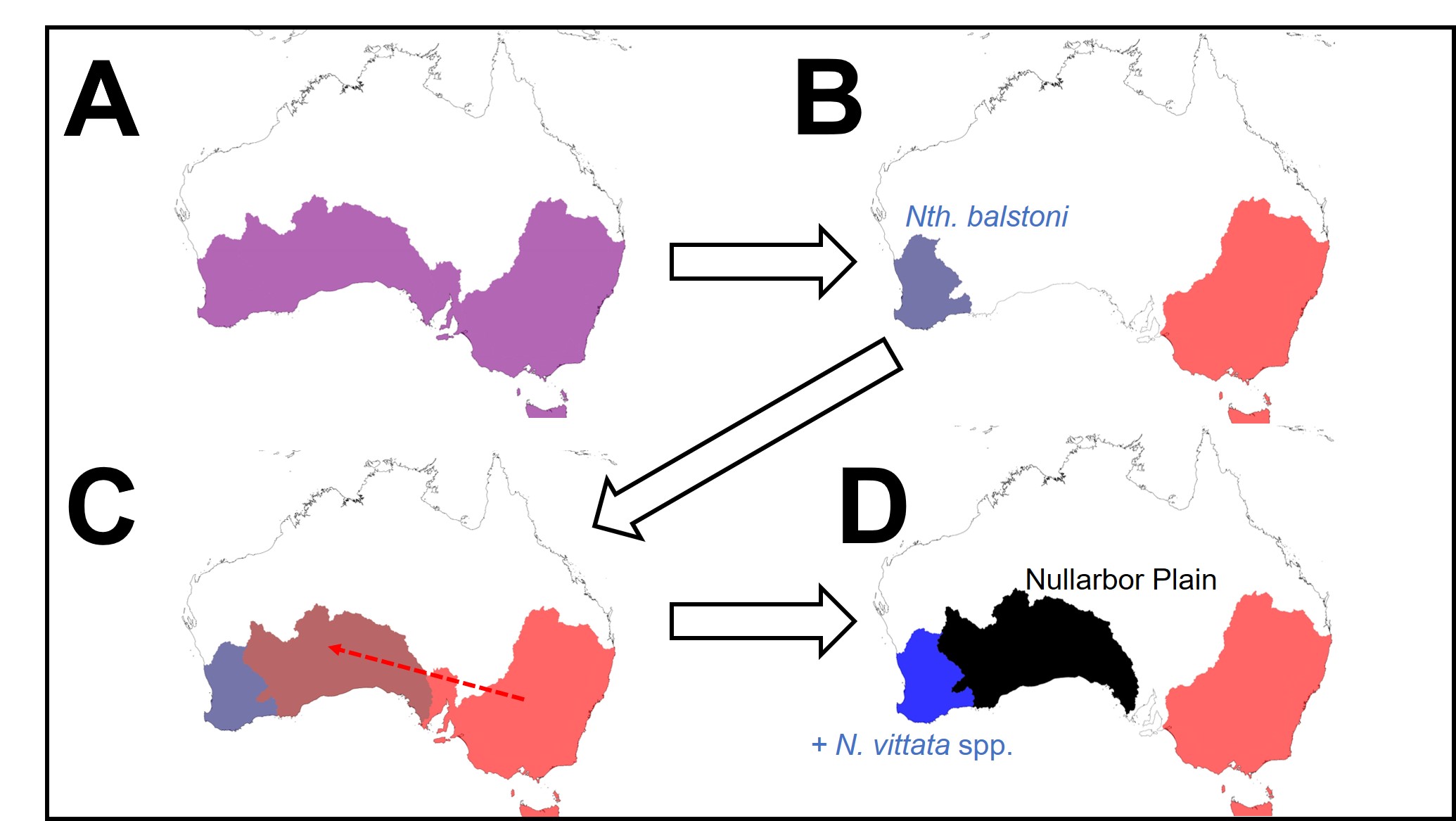
A diagram of the distribution of pygmy perch species over time, as suggested by the ancestral area reconstruction. A: the initial ancestor of pygmy perches was likely found throughout southern Australia. B: an unknown event splits the ancestor into an eastern and western group; the sole extant species of the W group is Nth. balstoni. C: the ancestor of the eastern pygmy perches spreads towards the west, entering part of the pre-Nullarbor region. D: due to changes in the hydrology of the area, some eastern pygmy perches (the maroon colour in C) are pushed towards the west; these form N. vittata species and N. pygmaea. The Nullarbor Plain forms and effectively cuts off the two groups from one another, isolating them.
What does this mean for pygmy perches?
Nearly all species of pygmy perch are threatened or worse in the conservation legislation; there have been many conservation efforts to try and save the worst-off species from extinction. Pygmy perches provide a unique insight to the history of the Australian climate and may be a key in unlocking some of the mysteries of what our land was like so long ago. Every species is important for conservation and even those small, hard-to-notice creatures that we might forget about play a role in our environmental history.