Drifting or driving: directionality in evolution

How random is evolution?

Often, we like to think of evolution fairly anthropomorphically; as if natural selection actively decides what is, and what isn’t, best for the evolution of a species (or population). Of course, there’s not some explicit Evolution God who decrees how a species should evolve, and in reality, evolution reflects a more probabilistic system. Traits that give a species a better chance of reproducing or surviving, and can be inherited by the offspring, will over time become more and more dominant within the species; contrastingly, traits that do the opposite will be ‘weeded out’ of the gene pool as maladaptive organisms die off or are outcompeted by more ‘fit’ individuals. The fitness value of a trait can be determined from how much the frequency of that trait varies over time.

So, if natural selection is just probabilistic, does this mean evolution is totally random? Is it just that traits are selected based on what just happens to survive and reproduce in nature, or are there more direct mechanisms involved? Well, it turns out both processes are important to some degree. But to get into it, we have to explain the difference between genetic drift and natural selection (we’re assuming here that our particular trait is genetically determined).  

Allele frequency over time diagram
The (statistical) overview of natural selection. In this example, we have two different traits in a population; the blue and the red O. Our starting population is 20 individuals (N), with 10 of each trait (a 1:1 ratio, or 50% frequency of each). We’re going to assume that, because the blue is favoured by natural selection, it doubles in frequency each generation (i.e. one individual with the blue has two offspring with one blue each). The red is neither here nor there and is stable over time (one red O produces one red O in the next generation). So, going from Gen 1 to Gen 2, we have twice as many blue Xs (Nt) as we did previously, changing the overall frequency of the traits (highlighted in yellow). Because populations probably don’t exponentially increase every generation, we’ll cut it back down to our original total of 20, but at the same ratios (Np). Over time, we can see that the population gradually accumulates more blue Xs relative to red Os, and by Gen 5 the red is extinct. Thus, the blue X has evolved!

When we consider the genetic variation within a species to be our focal trait, we can tell that different parts of the genome might be more related with natural selection than others. This makes sense; some mutations in the genome will directly change a trait (like fur colour) which might have a selective benefit or detriment, while others might not change anything physically or change traits that are neither here-nor-there under natural selection (like nose shape in people, for example). We can distinguish between these two by talking about adaptive or neutral variation; adaptive variation has a direct link to natural selection whilst neutral variation is predominantly the product of genetic drift. Depending on our research questions, we might focus on one type of variation over the other, but both are important components of evolution as a whole.

Genetic drift

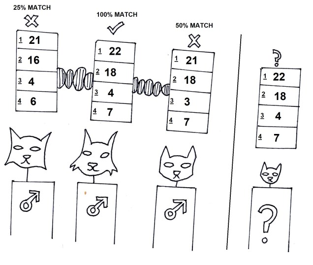
Genetic drift is considered the random, selectively ‘neutral’ changes in the frequencies of different traits (alleles) over time, due to completely random effects such as random mutations or random loss of alleles. This results in the neutral variation we can observe in the gene pool of the species. Changes in allele frequencies can happen due to entirely stochastic events. If, by chance, all of the individuals with the blue fur variant of a gene are struck by lightning and die, the blue fur allele would end up with a frequency of 0 i.e. go extinct. That’s not to say the blue fur ‘predisposed’ the individuals to be struck be lightning (we assume here, anyway), so it’s not like it was ‘targeted against’ by natural selection (see the bottom figure for this example).

Because neutral variation appears under a totally random, probabilistic model, the mathematical basis of it (such as the rate at which mutations appear) has been well documented and is the foundation of many of the statistical aspects of molecular ecology. Much of our ability to detect which genes are under selection is by seeing how much the frequencies of alleles of that gene vary from the neutral model: if one allele is way more frequent than you’d expect by random genetic drift, then you’d say that it’s likely being ‘pushed’ by something: natural selection.

Manhattan plot example
A Manhattan plot, which measures the level of genetic differentiation between two different groups across the genome. The x-axis shows the length of the genome, in this example colour-coded by the specific chromosome of the sequence, while the y-axis shows the level of differentiation between the two groups being studied. The dots represent certain spots (loci, singular locus) in the genome, with the level of differentiation (Fst) measured for that locus in one group vs that locus in the other group. The dotted line represents the ‘average differentiation’: i.e. how different you’d expect the two groups to be by chance. Anything about that line is significantly different between the two groups, either because of drift or natural selection. This plot has been slightly adapted from Axelsson et al. (2013), who were studying domestication in dogs by comparing the genetic architecture of wild wolves versus domestic dogs. In this example we can see that certain regions of the genome are clearly different between dogs and wolves (circled); when the authors looked at the genes within those blocks, they found that many were related to behavioural changes (nervous system), competitive breeding (sperm-egg recognition) and interestingly, starch digestion. This last category suggests that adaptation to an omnivorous diet (likely human food waste) was key in the domestication process.

Natural selection

Contrastingly to genetic drift, natural selection is when particular traits are directly favoured (or unfavoured) in the environmental context of the population; natural selection is very specific to both the actual trait and how the trait works. A trait is only selected for if it conveys some kind of fitness benefit to the individual; in evolutionary genetics terms, this means it allows the individual to have more offspring or to survive better (usually).

While this might be true for a trait in a certain environment, in another it might be irrelevant or even have the reverse effect. Let’s again consider white fur as our trait under selection. In an arctic environment, white fur might be selected for because it helps the animal to camouflage against the snow to avoid predators or catch prey (and therefore increase survivability). However, in a dense rainforest, white fur would stand out starkly against the shadowy greenery of the foliage and thus make the animal a target, making it more likely to be taken by a predator or avoided by prey (thus decreasing survivability). Thus, fitness is very context-specific.

Who wins? Drift or selection?

So, which is mightier, the pen (drift) or the sword (selection)? Well, it depends on a large number of different factors such as mutation rate, the importance of the trait under selection, and even the size of the population. This last one might seem a little different to the other two, but it’s critically important to which process governs the evolution of the species.

In very small populations, we expect genetic drift to be the stronger process. Natural selection is often comparatively weaker because small populations have less genetic variation for it to act upon; there are less choices for gene variants that might be more beneficial than others. In severe cases, many of the traits are probably very maladaptive, but there’s just no better variant to be selected for; look at the plethora of physiological problems in the cheetah for some examples.

Genetic drift, however, doesn’t really care if there’s “good” or “bad” variation, since it’s totally random. That said, it tends to be stronger in smaller populations because a small, random change in the number or frequency of alleles can have a huge effect on the overall gene pool. Let’s say you have 5 cats in your species; they’re nearly extinct, and probably have very low genetic diversity. If one cat suddenly dies, you’ve lost 20% of your species (and up to that percentage of your genetic variation). However, if you had 500 cats in your species, and one died, you’d lose only <0.2% of your genetic variation and the gene pool would barely even notice. The same applies to random mutations, or if one unlucky cat doesn’t get to breed because it can’t find a mate, or any other random, non-selective reason. One way we can think of this is as ‘random error’ with evolution; even a perfectly adapted organism might not pass on its genes if it is really unlucky. A bigger sample size (i.e. more individuals) means this will have less impact on the total dataset (i.e. the species), though.

Drift in small pops
The effect of genetic drift on small populations. In this example, we have two very similar populations of cats, each with three different alleles (black, blue and green) in similar frequencies across the populations. The major difference is the size of the population; the left is much smaller (5 cats) compared to the right (20 cats). If one cat randomly dies from a bolt of lightning (RIP), and assuming that the colour of the cat has no effect on the likelihood of being struck by lightning (i.e. is not under natural selection), then the outcome of this event is entirely due to genetic drift. In this case, the left population has lost 1/5th of its population size and 1/3rd of its total genetic diversity thanks to the death of the genetically unique blue cat (He will be missed) whereas the right population has only really lost 1/20th of its size and no changes in total diversity (it’ll recover).

Both genetic drift and natural selection are important components of evolution, and together shape the overall patterns of evolution for any given species on the planet. The two processes can even feed into one another; random mutations (drift) might become the genetic basis of new selective traits (natural selection) if the environment changes to suit the new variation. Therefore, to ignore one in favour of the other would fail to capture the full breadth of the processes which ultimately shape and determine the evolution of all species on Earth, and thus the formation of the diversity of life.

“Who Do You Think You Are?”: studying the evolutionary history of species

The constancy of evolution

Evolution is a constant, endless force which seeks to push and shape species based on the context of their environment: sometimes rapidly, sometimes much more gradually. Although we often think of discrete points of evolution (when one species becomes two, when a particular trait evolves), it is nevertheless a continual force that influences changes in species. These changes are often difficult to ‘unevolve’ and have a certain ‘evolutionary inertia’ to them; because of these factors, it’s often critical to understand how a history of evolution has generated the organisms we see today.

What do I mean when I say evolutionary history? Well, the term is fairly diverse and can relate to the evolution of particular traits or types of traits, or the genetic variation and changes related to these changes. The types of questions and points of interest of evolutionary history can depend at which end of the timescale we look at: recent evolutionary histories, and the genetics related to them, will tell us different information to very ancient evolutionary histories. Let’s hop into our symbolic DeLorean and take a look back in time, shall we?

Labelled_evolhistory
A timeslice of evolutionary history (a pseudo-phylogenetic tree, I guess?), going from more recent history (bottom left) to deeper history (top right). Each region denoted in the tree represents the generally area of focus for each of the following blog headings. 1: Recent evolutionary history might look at individual pedigrees, or comparing populations of a single species. 2: Slightly older comparisons might focus on how species have arisen, and the factors that drive this (part of ‘phylogeography’). 3: Deep history might focus on the origin of whole groups of organisms and a focus on the evolution of particular traits like venom or sociality.

Very recent evolutionary history: pedigrees and populations

While we might ordinarily consider ‘evolutionary history’ to refer to events that happened thousands or millions of years ago, it can still be informative to look at history just a few generations ago. This often involves looking at pedigrees, such as in breeding programs, and trying to see how very short term and rapid evolution may have occurred; this can even include investigating how a particular breeding program might accidentally be causing the species to evolve to adapt to captivity! Rarely does this get referred to as true evolutionary history, but it fits on the spectrum, so I’m going to count it. We might also look at how current populations are evolving differently to one another, to try and predict how they’ll evolve into the future (and thus determine which ones are most at risk, which ones have critically important genetic diversity, and the overall survivability of the total species). This is the basis of ‘evolutionarily significant units’ or ESUs which we previously discussed on The G-CAT.

Captivefishcomic
Maybe goldfish evolved 3 second memory to adapt to the sheer boringness of captivity? …I’m joking, of course: the memory thing is a myth and adaptation works over generations, not a lifetime.

A little further back: phylogeography and species

A little further back, we might start to look at how different populations have formed or changed in semi-recent history (usually looking at the effect of human impacts: we’re really good at screwing things up I’m sorry to say). This can include looking at how populations have (or have not) adapted to new pressures, how stable populations have been over time, or whether new populations are being ‘made’ by recent barriers. At this level of populations and some (or incipient) species, we can find the field of ‘phylogeography’, which involves the study of how historic climate and geography have shaped the evolution of species or caused new species to evolve.

Evolution of salinity
An example of trait-based phylogenetics, looking at the biogeographic patterns and evolution/migration to freshwater in perch-like fishes, by Chen et al. (2014). The phylogeny shows that a group of fishes adapted to freshwater environments (black) from a (likely) saltwater ancestor (white), with euryhaline tolerance evolving two separate times (grey).

One high profile example of phylogeographic studies is the ‘Out of Africa’ hypothesis and debate for the origination of the modern human species. Although there has been no shortage of debate about the origin of modern humans, as well as the fate of our fellow Neanderthals and Denisovans, the ‘Out of Africa’ hypothesis still appears to be the most supported scenario.

human phylogeo
A generalised diagram of the ‘Out of Africa’ hypothesis of human migration, from Oppenheimer, 2012. 

Phylogeography is also component for determining and understanding ‘biodiversity hotspots’; that is, regions which have generated high levels of species diversity and contain many endemic species and populations, such as tropical hotspots or remote temperate regions. These are naturally of very high conservation value and contribute a huge amount to Earth’s biodiversity, ecological functions and potential for us to study evolution in action.

Deep, deep history: phylogenetics and the origin of species (groups)

Even further back, we start to delve into the more traditional concept of evolutionary history. We start to look at how species have formed; what factors caused them to become new species, how stable the new species are, and what are the genetic components underlying the change. This subfield of evolution is called ‘phylogenetics’, and relates to understanding how species or groups of species have evolved and are related to one another.

Sometimes, this includes trying to look at how particular diagnostic traits have evolved in a certain group, like venom within snakes or eusocial groups in bees. Phylogenetic methods are even used to try and predict which species of plants might create compounds which are medically valuable (like aspirin)! Similarly, we can try and predict how invasive a pest species may be based on their phylogenetic (how closely related the species are) and physiological traits in order to safeguard against groups of organisms that are likely to run rampant in new environments. It’s important to understand how and why these traits have evolved to get a good understanding of exactly how the diversity of life on Earth came about.

evolution of venom
An example of looking at trait evolution with phylogenetics, focusing on the evolution of venom in snakes, from Reyes-Velasco et al. (2014). The size of the boxes demonstrates the number of species in each group, with the colours reflecting the number of venomous (red) vs. non-venomous (grey) species. The red dot shows the likely origin of venom.

Phylogenetics also allows us to determine which species are the most ‘evolutionarily unique’; all the special little creatures of plant Earth which represent their own unique types of species, such as the tuatara or the platypus. Naturally, understanding exactly how precious and unique these species are suggests we should focus our conservation attention and particularly conserve them, since there’s nothing else in the world that even comes close!

Who cares what happened in the past right? Well, I do, and you should too! Evolution forms an important component of any conservation management plan, since we obviously want to make sure our species can survive into the future (i.e. adapt to new stressors). Trying to maintain the most ‘evolvable’ groups, particularly within breeding programs, can often be difficult when we have to balance inbreeding depression (not having enough genetic diversity) with outbreeding depression (obscuring good genetic diversity by adding bad genetic diversity into the gene pool). Often, we can best avoid these by identifying which populations are evolutionarily different to one another (see ESUs) and using that as a basis, since outbreeding vs. inbreeding depression can be very difficult to measure. This all goes back to the concept of ‘adaptive potential’ that we’ve discussed a few times before.

In any case, a keen understanding of the evolutionary trajectory of a species is a crucial component for conservation management and to figure out the processes and outcomes of evolution in the real world. Thus, evolutionary history remains a key area of research for both conservation and evolution-related studies.


What’s the story with these little fish?

The pygmy perches

I’ve mentioned a few times in the past that my own research centres around a particular group of fish: the pygmy perches. When I tell people about them, sometimes I get the question “why do you want to study them?” And to be fair, it’s a good question: there must be something inherently interesting about them to be worth researching. And there is plenty.

Pygmy perches are a group of very small (usually 4-6cm) freshwater fish native to temperate Australia: they’re found throughout the southwest corner of WA and the southeast of Australia, stretching from the mouth of the Murray River in SA up to lower Queensland (predominantly throughout the Murray-Darling Basin) and even in northern Tasmania. There’s a massive space in the middle where they aren’t found: this is the Nullarbor Plain, and is a significant barrier for nearly all freshwater species (since it holds practically no water).

Unmack_distributions
The distributions of different pygmy perch species (excluding Bostockia porosa, which is a related but different group), taken from Unmack et al. (2011). The black region in the bottom right part indicates the Nullarbor Plain, which separates eastern and western species.

The group consists of 2 genera (Nannoperca and Nannatherina) and 7 currently described species, although there could be as many as 10 actual species (see ‘cryptic species’: I’ll elaborate on this more in future posts…). They’re very picky about their habitat, preferring to stay within low flow waterbodies with high vegetation cover, such as floodplains and lowland creeks. Most species have a lifespan of a couple years, with different breeding times depending on the species.

Why study pygmy perches?

So, they’re pretty cute little fish. But unfortunately, that’s not usually enough justification to study a particular organism. So, why does the Molecular Ecology Lab choose to use pygmy perch as one (of several) focal groups? Well, there’s a number of different reasons.

The main factors that contribute to their research interest are their other characteristics: because they’re so small and habitat specialists, they often form small, isolated populations that are naturally separated by higher flow rivers and environmental barriers. They also appear to have naturally very low genetic diversity: ordinarily, we’d expect that they wouldn’t be great at adapting and surviving over a long time. Yet, they’ve been here for a long time: so how do they do it? That’s the origin of many of the research questions for pygmy perches.

Adaptive evolution despite low genetic variation

One of the fundamental aspects of the genetic basis of evolution is the connection between genetic diversity and ‘adaptability’: we expect that populations or species with more genetic diversity are much more likely to be able to evolve and adapt to new selective pressures than those without it. Pygmy perches clearly contradict this at least a little bit, and so much of the research in the lab is about understanding exactly what factors and mechanisms contribute to the ability of pygmy perches to apparently adapt and survive what is traditionally not consider a very tolerant place to live. Recent research suggests the different expression of genes may be an important mechanism of adaptation for pygmy perch.

Recommended readings: Brauer et al. (2016); Brauer et al. (2017).

The influence of the historic environment on evolution

From an evolutionary standpoint, pygmy perches are unique in more ways than just their genetic diversity. They’re relatively ancient, with the origin of the group estimated at around 40 million years ago. Since then, they’ve diversified into a number of different species and have spread all over the southern half of the Australian continent, demonstrating multiple movements across Australia in that time. This pattern is unusual for freshwater organisms, and this combined with their ancient nature makes them ideal candidates for studying the influence of historic environment, climate and geology on the evolution and speciation of freshwater animals in Australia. And that’s the focus of my PhD (although not exclusively; plenty of other projects have explored questions in this area).

Bass Strait timelapse
The changing sea levels across the Bass Strait from A) 25 thousand years ago, B) 17.5 thousand years ago, and C) 14 thousand years ago (similar to today), from Lambeck and Chappel (2001). This is an example of one kind of environmental change that would likely have influenced the evolutionary patterns of pygmy perch, separating the populations from northern Tasmania and Victoria.

Recommended readings: Unmack et al. (2013); Unmack et al. (2011).

Conservation management and ecological role

Of course, it’s all well and good to study the natural, evolutionary history of an organism as if it hasn’t had any other influences. But we all know how dramatic the impact humans have on the environment are and unfortunately for many pygmy perch species this means that they are threatened or endangered and at risk of extinction. Their biggest threats are introduced predators (such as the redfin perch and European carp), alteration of waterways (predominantly for agriculture) and of course, climate change. For some populations, local extinction has already happened: some populations of the Yarra pygmy perch (N. obscura) are now completely gone from the wild. Many of these declines occurred during the Millennium Drought, where the aforementioned factors were exacerbated by extremely low water availability and consistently high temperatures. So naturally, a significant proportion of the work on pygmy perches is focused on their conservation, and trying to boost and recover declining populations.

This includes the formation of genetics-based breeding programs for two species, the southern pygmy perch and Yarra pygmy perch. A number of different organisations are involved in this ongoing process, including a couple of schools! These programs are informed by our other studies of pygmy perch evolution and adaptive potential and hopefully combined we can save these species from becoming totally extinct.

Yarra-breeders-vid.gif
Some of the Yarra pygmy perch from the extinct Murray-Darling Basin population, ready to make breeding groups!
Fin clipping Yarras.jpg
Me, fin clipping the Yarra pygmy perch in the breeding groups for later genetic analyses. Yes, I know, I needed a haircut.

Recommended readings: Brauer et al. (2013); Attard et al. (2016); Hammer et al. (2013).

Hopefully, some of this convinces you that pygmy perch are actually rather interesting creatures (I certainly think so!). Pygmy perch research can offer a unique insight into evolutionary history, historical biogeography, and conservation management. Also, they’re kinda cute….so that’s gotta count for something, right? If you wanted to find out more about pygmy perch research, and get updates on our findings, be sure to check out the Molecular Ecology Lab Facebook page or our website!

Bigger and better: the evolution of genomic markers

From genetic to genomic markers

As we discussed in last week’s post, different parts of the DNA can be used as genetic markers for analyses relating to conservation, ecology and evolution. We looked at a few different types of markers (allozymes, microsatellites, mitochondrial DNA) and why different markers are good for different things. This week, we’ll focus on the much grander and more modern state of genomics; that is, using DNA markers that are often thousands of genes big!

Genomics vs genetics
If we pretended that the size of the text for each marker was indicative of how big the data is, this figure would probably be about a 1000x under-estimation of genomic datasets. There is not enough room on the blog page to actually capture this.

I briefly mentioned last week that the development of genomics was largely facilitated by what we call ‘next-generation sequencing’, which allows us to easily obtain billions of fragments of DNA and collate them into a useful dataset. Most genomic technologies differ based on how they fragment the DNA for sequencing and how the data is processed.

While the analytical, monetary and time cost of obtaining genomic data has decreased as sequencing technology has improved, we still need to balance these factors together when deciding which method to use. Many methods allow us to put many individual samples together in the same reaction (we tell which sequence belongs to which sequence using special ‘barcode sequences’ that code for one specific sample): in this case, we also need to consider how many samples to place together (“multiplex”).

As a broad generalisation, we can separate most genomic sequencing methods into two broad categories: whole genome or reduced-representation. As the name suggests, whole genome sequencing involves collecting the entire genome of the individuals we use, although this is generally very expensive and can only be done with a limited number of samples at a time. If we want to have a much larger dataset, often we’ll use reduced-representation methods: these involve breaking down the whole genome into much smaller fragments and as many of these as we can to get a broad overview of the genome. Reduced-representation methods are much cheaper and are appropriate for larger sample sizes than whole genome, but naturally lose large amounts of information from the genome.

Genomic sequencing pathway
The (very, very) vague outline of genomic sequencing. First we take all of the DNA of an organism, breaking it into smaller fragments in this case using a restriction enzyme (see below). We then amplify these fragments, making billions of copies of them before piecing them back together to either make the entire genome (left) of a few individuals or patches of the genome (right) for more individuals.

Restriction-site associated DNA (RADseq)

Within the Molecular Ecology Lab, we predominantly use a technology known as “double digest restriction site-associated DNA sequencing”, which is a huge mouthful so we just call it ‘ddRAD’. This sounds incredibly complicated, but (as far as sequencing methods go, anyway) is actually relatively simple. We take the genome of a sample, and then using particular enzymes (called ‘restriction enzymes’), we break the genome randomly down into small fragments (usually up to 200 bases long, after we filter it). We then attach a specific barcode for that individual, and a few more bits and pieces as part of the sequencing process, and then pool them together. This pool (a “library”) is sent off to a facility to be run through a sequencing machine and produce the data we work with. The ‘dd’ part of ‘ddRAD’ just means that a pair of restriction enzymes are used in this method, instead of just one (it’s a lot cleaner and more efficient).

ddRAD flowchart
A simplified standard ddRAD protocol. 1) We obtain the DNA-containing tissue of the organism we want to study, such as blood, skin or muscle samples. 2) We extract all of the genomic DNA from the tissue sample, making sure we have good quantity and quality (avoiding degradation if possible). 3) We break the genome down into smaller fragments using restriction enzymes, which cut at certain places (orange and green marks on the top line). We then attach special sequences to these fragments, such as the adapter (needed for the sequencer to work) and the barcode for that specific individual organism (the green bar). 4) We amplify the fragments, generating billions of copies of each of them. 5) We send these off to a sequencing facility to read the DNA sequence of these fragments (often outsourced to a private institution). 6) We get back a massive file containing all of the different sequences for all of the organisms in one file. 7) We separate out these sequences into the individual the came from by using their special barcode as an identifier (the coloured codes). 8) We then process this data to make sure it’s of the best quality possible, including removing sequences that we don’t have enough copies of or have errors. From this, we produce a final dataset, often with one continuous sequence for each individual. If this dataset doesn’t meet our standards for quality or quantity, we go back and try new filtering parameters.

Gene expression and transcriptomics

Sometimes, however, we might not even want to look at the exact DNA sequence. You might remember in an earlier blog post that I mentioned genes can be ‘switched on’ or ‘switched off’ by activator or repressor proteins. Well, because of this, we can have the exact same genes act in different ways depending on the environment. This is most observable in tissue development: although all of the cells of all of your organs have the exact same genome, the control of gene expression changes what genes are active and thus the physiology of the organ. We might also have genes which are only active in an organism under certain conditions, like heat shock proteins under hot conditions.

This can be an important part of evolution as being able to easily change genetic expression may allow an individual to adapt to new environmental pressures much more easily; we call this ‘phenotypic plasticity’. In this case, instead of sequencing the DNA, we might want to look at which genes are expressed, or how much they are expressed, in different conditions or populations: this is called ‘comparative transcriptomics’. So instead of sequencing the DNA, we sequence the RNA of an organism (the middle step of making proteins, so most RNAs are only present if the gene is being expressed).

Processing data

Despite how it must appear, most of the work with genomic datasets actually comes after you get the sequences back. Because of the nature and scale of genomic datasets, rigorous analytical pipelines are needed to manage and filter data from the billions of small sequences into full sequences of high quality. There are many different ways to do this, and usually involves playing with parameters, so I won’t delve into the details (although some of it is explained in the boxed part of the flowchart figure).

The future of genomics

No doubt as the technology improves, whole genome sequencing will become progressively more feasible for more species, opening up the doors for a new avalanche of data and possibilities. In any case, we’ve come a long way since the first whole genome (for Haemophilus influenzae) in 1995 and the construction of the whole human genome in 2003.


Using the ‘blueprint of life’: an introduction to DNA markers

What is a ‘molecular marker’?

As we’ve previously discussed within The G-CAT, information from the DNA of organisms can be used in a variety of ways to study evolution and ecology, inform conservation management, and understand the diversity of life on Earth. We’ve also had a look at the general background of the DNA itself, and some of the different parts of the genome. What we haven’t discussed yet is how we use the DNA sequence in these studies; most importantly, which part of the genome to use.

The genome of most organisms is massive. The size of the genome ranges depending on the organism, with one of the smallest recorded genomes belonging to a bacteria (Carsonella ruddi), consisting of 160,000 bases. There is a bit of debate about the largest recorded genome, but one contender (the ‘canopy plant’, Paris japonica) has a genome stretching 150 billion base pairs long! The human genome sits in the middle at around 3 billion bases long. Naturally, it would be incredibly difficult to obtain the sequence of the whole genome of many organisms (particularly 20 – 30 years ago, due to technological limitations in the sequencing process) so instead we usually pick a specific region of the genome instead. The exact region (or type of region) we use is referred to as a ‘molecular marker’.

How do we choose a good marker?

The marker we pick is incredibly important: this is often based on how much variation we need to observe across groups. For example, if we want to study differences between individuals, say in a pedigree analysis, we need to pick a section of the DNA that will show differences between individuals; it will need to mutate fairly rapidly to be useful. If it mutates too slowly, all individuals will look identical genetically and we won’t have learnt anything new at all.

On the flipside, if we want to study evolution at a larger scale (say, between species, or groups of species) we would need to use a marker that evolves much slower. Using a rapidly mutating section of DNA would effectively give a tonne of ‘white noise’; it’d be impossible to pick what is the genetic difference at the species level (i.e. one species is different to another at that base) vs. at the individual level (i.e. one or many individuals within the species are different). Thus, we tend to use much slower mutating markers for deeper evolutionary history.

Evol spectrum
The spectrum of evolutionary history, with evolutionary splits between major animal groups on the left, to splits between species in the middle, to splits between individuals within a family tree on the right. The effectiveness of a marker for a particular part of the spectrum depends on its mutation rate. The original figure was taken from a landmark paper by Avise (1994), considered one of the forefathers of molecular ecology.

Think of it like comparing cats and dogs. If we wanted to compare different cats to one another (say different breeds) we could use hair length or coat colour as a useful trait. Since some breeds have different coat characteristics, and these don’t vary as much within the breed as across breeds, we can easily determine a long haired cat from a short haired cat. However, if we tried to use coat colour and length to compare cats and dogs we’d be stumped, because both species have lots of variation in these traits within their species. Some cats have coat length more similar to some dogs than to other cats for example; so they’re not a good characteristics to separate the two animal species (we might use muzzle shape, or body shape instead). If we substitute each of these traits with a particular marker, then we can see that some markers are better for some comparisons but not good for others.

Allozymes

The most traditional molecular marker are referred to as ‘allozymes’; instead of comparing actual genetic sequences (something that was not readily possible early in the field), variations in the shape (i.e. the amino acids of the protein, not the code underlying it) were compared between species. Changes in proteins occur very rarely as natural selection tends to push against randomly changing protein structure, since the shape of it is critical to its function and functionality. Because of this, allozymes were only really effective for studying very broad comparisons (mainly across species or species groups); the exact protein used depends on the study organism. Allozymes are generally considered outdated in the field nowadays.

With the development of technologies that allowed us to actual determine the DNA code of genes, molecular ecology moved into comparing actual sequences across individuals. However, early sequencing technology could generally only accurately determine small sections of DNA at a time, so particular markers capitalising on this were developed. Many of these are still used due to their cost-effectiveness and general ease of analysing.

Microsatellites

For comparing closely related individuals (within a pedigree, or a population), markers called ‘microsatellites’ are widely used. These are small sections of the genome which have repetitive DNA codes; usually, the same two or three base pairs (one ‘motif’) are repeated a number of times afterwards (the ‘repeat number’). While the motifs themselves rarely get mutations, the number of repeated motifs very rapidly mutates. This is because the protein that copies DNA is not very perfect, and often ‘slips up’, and adds or cuts off a repeat from the microsatellite sequence. Thus, differences in the repeat number of microsatellites accumulate pretty quickly, to the point where you can determine the parents of an individual with them.

Microsat_diagram
The general (and simplified) structure of a microsatellite marker. 

Microsatellites are often used in comparisons across closely related individuals, such as within pedigrees or within populations. While they are relatively easy to obtain, one drawback is that you need to have some understanding of the exact microsatellite you wish to analyse before you start; you need to make a specific ‘primer’ sequence to be able to get the right marker, as some may not be informative in particular species or comparisons. Many researchers choose to use 10-20 different microsatellite markers together in these types of studies, such as in human parentage analyses.

Cats_parentage
Microsatellites are useful for parentage analysis. Our previous guest contestants are here to discuss ‘Who is the father?!’ in Maury-like fashion. The results are in, and using 4 microsatellites (1-4) and looking at the number of repeats in each of those, we can see the contestant 2 is undoubtedly the father! I’ll be honest, I have no idea if this is how Maury works, but I think it would work.

Mitochondrial DNA

For deeper comparisons, however, microsatellites mutate far too rapidly to be effective. Instead, we can choose to use the DNA of the mitochondria. You may remember the mitochondria as ‘the powerhouse of the cell’; while this is true, it also has a lot of other unique properties. The mitochondria was actually (a very, very, very long time ago) a separate bacteria-like organism which became symbiotically embedded within another cell. Because of this, and despite a couple billion years of evolution since that time, the mitochondria actually has its own genome separate to the ‘host’ (like the standard human genome). The full mitochondrial genome consists of around 37 different genes, most of which don’t code for any proteins involved directly in evolution; as such, natural selection doesn’t affect them as much as other genes. The most commonly used mitochondrial genes are the cytochrome b oxidase gene (cytb for short) or the cytochrome c oxidase 1 (CO1) gene.

The mitochondrial genome evolves relatively rapidly (but not nearly as fast as microsatellites) and is found in pretty much every plant and animal on the planet. Because of these traits, it’s often used as a way of diagnosing species through the ‘Barcode of Life’ project (using cytb and CO1). It’s very widely used within species-level studies, to the point where we can even use the relatively consistent mutation rate of the mitochondrial genome to estimate how long ago different species separated in evolution.

Cats_barcode
Not entirely how the Barcode of Life works, but close enough, right?

Other markers?

There are plenty of other genetic markers that are used within molecular ecology, with some focusing on only the exons or introns of genes, or other repetitive sequences. However, microsatellites and mitochondrial genes are among the most widely used in evolution and conservation studies.

While these markers have been very useful in building the foundations of molecular ecology as a scientific field, developments in sequencing technology, analytical methods and evolutionary theory have pushed our ability to use DNA to understand evolution and conservation even further. Particularly the development of sequencing machines which can process much larger amounts of genetic DNA. This has pushed genetics into the age of ‘genomics’: while this sounds like a massively technical difference, it’s really just about the difference in the size of the data we can use. Obviously, this has many other benefits for the kinds of questions we can ask about evolution, conservation and ecology.

Genomics has massively expanded in recent years, the types, quantity and quality of data are diverse. Stay tuned because next week, we’ll start to delve into the modern world of genomics!