The idea of using the genetic sequences of living organisms to understand the evolutionary history of species is a concept much repeated on The G-CAT. And it’s a fundamental one in phylogenetics, taxonomy and evolutionary biology. Often, we try to analyse the genetic differences between individuals, populations and species in a tree-like manner, with close tips being similar and more distantly separated branches being more divergent. However, this runs on one very key assumption; that the patterns we observe in our study genes matches the overall patterns of species evolution. But this isn’t always true, and before we can delve into that we have to understand the difference between a ‘gene tree’ and a ‘species tree’.
A gene tree or a species tree?
Our typical view of a phylogenetic tree is actually one of a ‘gene tree’, where we analyse how a particular gene (or set of genes) have changed over time between different individuals (within and across populations or species) based on our understanding of mutation and common ancestry.
However, a phylogenetic tree based on a single gene only demonstrates the history of that gene. What we assume in most cases is that the history of that gene matches the history of the species: that branches in the genetic tree mirror when different splits in species occurred throughout history.
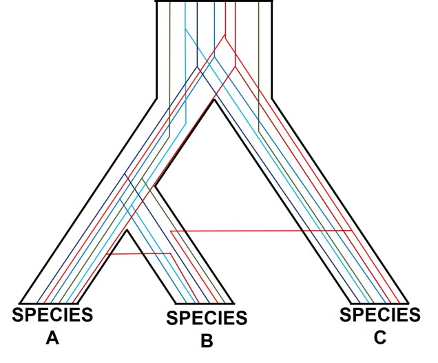
The easiest way to conceptualise gene trees and species trees is to think of individual gene trees that are nested within an overarching species tree. In this sense, individual gene trees can vary from one another (substantially, even) but by looking at the overall trends of many genes we can see how the genome of the species have changed over time.
A (potentially familiar) depiction of individual gene trees (coloured lines) within the broader species tree (defined b the black boundaries). As you might be able to tell, the branching patterns of the different genes are not the same, and don’t always match the overarching species tree.
One of the most prolific, but more complicated, ways gene trees can vary from their overarching species tree is due to what we call ‘incomplete lineage sorting’. This is based on the idea that species and the genes that define them are constantly evolving over time, and that because of this different genes are at different stages of divergence between population and species. If we imagine a set of three related populations which have all descended from a single ancestral population, we can start to see how incomplete lineage sorting could occur. Our ancestral population likely has some genetic diversity, containing multiple alleles of the same locus. In a true phylogenetic tree, we would expect these different alleles to ‘sort’ into the different descendent populations, such that one population might have one of the alleles, a second the other, and so on, without them sharing the different alleles between them.
If this separation into new populations has been recent, or if gene flow has occurred between the populations since this event, then we might find that each descendent population has a mixture of the different alleles, and that not enough time has passed to clearly separate the populations. For this to occur, sufficient time for new mutations to occur and genetic drift to push different populations to differently frequent alleles needs to happen: if this is too recent, then it can be hard to accurately distinguish between populations. This can be difficult to interpret (see below figure for a visualisation of this), but there’s a great description of incomplete lineage sorting here.
A demonstration of incomplete lineage sorting, generously adapted from a talk by fellow MELFU postdocs Dr Yuma (Jonathon) Sandoval-Castillo and Dr Catherine Attard. On the left is a depiction of a single gene coalescent tree over time: circles represent a single individual at a particular point in time (row) with the colours representing different alleles of that same gene. The tree shows how new mutations occur (colour changes along the branches) and spread throughout the descendent populations. In this example, we have three recently separated species, with a good number of different alleles. However, when we study these alleles in tree form (the phylogeny on the right), we see that the branches themselves don’t correlate well with the boundaries of the species. For example, the teal allele found within Species C is actually more similar to Species B alleles (purple and blue) than any other Species B alleles, based on the order and patterns of these mutations.
Hybridisation and horizontal transfer
Another way individual genes may become incongruent with other genes is through another phenomenon we’ve discussed before: hybridisation (or more specifically, introgression). When two individuals from different species breed together to form a ‘hybrid’, they join together what was once two separate gene pools. Thus, the hybrid offspring has (if it’s a first generation hybrid, anyway) 50% of genes from Species A and 50% of genes from Species B. In terms of our phylogenetic analysis, if we picked one gene randomly from the hybrid, we have 50% of picking a gene that reflects the evolutionary history of Species A, and 50% chance of picking a gene that reflects the evolutionary history of Species B. This would change how our outputs look significantly: if we pick a Species A gene, our ‘hybrid’ will look (genetically) very, very similar to Species A. If we pick a Species B gene, our ‘hybrid’ will look like a Species B individual instead. Naturally, this can really stuff up our interpretations of species boundaries, distributions and identities.
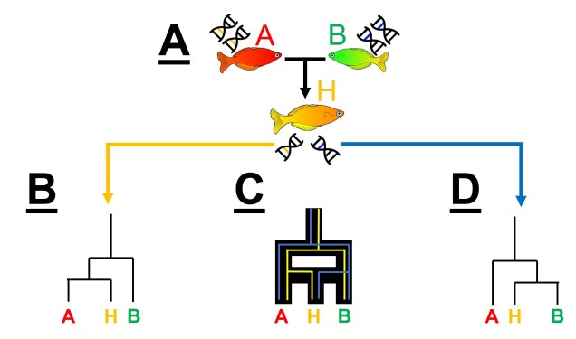
An example of hybridisation leading to gene tree incongruence with our favourite colourful fish. A) We have a hybridisation event between a red fish (Species A) and a green fish (Species B), resulting in a hybrid species (‘Species’ H). The red fish genome is indicated by the yellow DNA, the green fish genomes by the blue DNA, and the hybrid orange fish has a mixture of these two. B) If we sampled one set of genes in the hybrid, we might select a gene that originated from the red fish, showing that the hybrid is identical (or very similar) the Species A. D) Conversely, if we sampled a gene originating from the green fish, the resultant phylogeny might show that the hybrid is the same as Species B. C) If we consider these two patterns in combination, which see the true pattern of species formation, which is not a clear dichotomous tree and rather a mixture of the two sets of trees.
This can have a profound impact as paralogous genes are difficult to detect: if there has been a gene duplication early in the evolutionary history of our phylogenetic tree, then many (or all) of our study samples will have two copies of said gene. Since they look similar in sequence, there’s all possibility that we pick Variant 1 in some species and Variant 2 in other species. Being unable to tell them apart, we can have some very weird and abstract results within our tree. Most importantly, different samples with the same duplicated variant will seem similar to one another (e.g. have evolved from a common ancestor more recently) than it will to any sample of the other variant (even if they came from the exact same species)!
An example of how paralogous genes can confound species tree. We start with a single (purple) gene: at a particular point in time, this gene duplicates into a red and a blue form. Each of these genes then evolve and spread into four separate descendent species (A, B, C and D) but not in entirely the same way. However, since both the red and blue genetic sequences are similar, if we took a single gene from each species we might (somewhat randomly) sequence either the red or the blue copy. The different phylogenetic trees on the right demonstrate how different combinations of red and blue genes give very different patterns, since all blue copies will be more related to other blue genes than to the red gene of the same species. E.g. a blueA and a blueC are more similar than a blueA and a redA.
Overcoming incongruence with genomics
Although a tricky conundrum in phylogenetics and evolutionary genetics broadly, gene tree incongruence can largely be overcome with using more loci. As the random changes of any one locus has a smaller effect of the larger total set of loci, the general and broad patterns of evolutionary history can become clearer. Indeed, understanding how many loci are affected by what kind of process can itself become informative: large numbers of introgressed loci can indicate whether hybridisation was recent, strong, or biased towards one species over another, for example. As with many things, the genomic era appears poised to address the many analytical issues and complexities of working with genetic data.
Given the strong influence of genetic identity on the process and outcomes of the speciation process, it seems a natural connection to use genetic information to study speciation and species identities. There is a plethora of genetics-based tools we can use to investigate how speciation occurs (both the evolutionary processes and the external influences that drive it). One clear way to test whether two populations of a particular species are actually two different species is to investigate genes related to reproductive isolation: if the genetic differences demonstrate reproductive incompatibilities across the two populations, then there is strong evidence that they are separate species (at least under the Biological Species Concept; see Part One for why!). But this type of analysis requires several tools: 1) knowledge of the specific genes related to reproduction (e.g. formation of sperm and eggs, genital morphology, etc.), 2) the complete and annotated genome of the species (to be able to find and analyse the right genes properly) and 3) a good amount of data for the populations in question. As you can imagine, for people working on non-model species (i.e. ones that haven’t had the same history and detail of research as, say, humans and mice), this can be problematic. So, instead, we can use other genetic information to investigate and suggest patterns and processes related to the formation of new species.
Is reproductive isolation naturally selected for or just a consequence?
A fundamental aspect of studies of speciation is a “chicken or the egg”-type paradigm: does natural selection directly select for rapid reproductive isolation, preventing interbreeding; or as a secondary consequence of general adaptive differences, over a long history of evolution? This might be a confusing distinction, so we’ll dive into it a little more.
Of the two proposed models of speciation, the by-product of natural selection (the second model) has been the more favoured. Simply put, this expands on Darwin’s theory of evolution that describes two populations of a single species evolving independently of one another. As these become more and more different, both in physical (‘phenotype’) and genetic (‘genotype’) characteristics, there comes a turning point where they are so different that an individual from one population could not reasonably breed with an individual from the other to form a fertile offspring. This could be due to genetic incompatibilities (such as different chromosome numbers), physiological differences (such as changes in genital morphology), or behavioural conflicts (such as solitary vs. group living).
Certainly, this process makes sense, although it is debatable how fast reproductive isolation would occur in a given species (or whether it is predictable just based on the level of differentiation between two populations). Another model suggests that reproductive isolation actually might arise very quickly if natural selection favours maintaining particular combinations of traits together. This can happen if hybrids between two populations are not particularly well adapted (fit), causing natural selection to favour populations to breed within each group rather than across groups (leading to reproductive isolation). Typically, this is referred to as ‘reinforcement’ and predominantly involves isolating mechanisms that prevent individuals across populations from breeding in the first place (since this would be wasted energy and resources producing unfit offspring). The main difference between these two models is the sequence of events: do populations ecologically diverge, and because of that then become reproductively isolated, or do populations selectively breed (enforcing reproductive isolation) and thus then evolve independently?
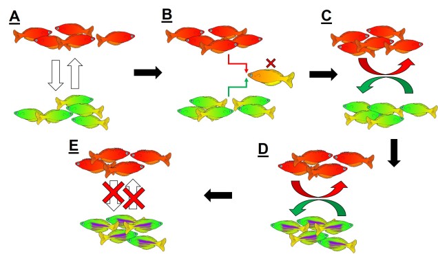
An example of reinforcement leading to speciation. A) We start with two populations of a single species (a red fish population and a green fish population), which can interbreed (the arrows). B) Because these two groups can breed, hybrids of the two populations can be formed. However, due to the poor combination of red and green fish genes within a hybrid, they are not overly fit (the red cross). C) Since natural selection doesn’t favour forming hybrids, populations then adapt to selectively breed only with similar fish, reducing the amount of interbreeding that occurs. D) With the two populations effectively isolated from one another, different adaptations specific to each population (spines in red fish, purple stripes in green fish) can evolve, causing them to further differentiate. E) At some point in the differentiation process, hybrids move from being just selectively unfit (as in B)) to entirely impossible, thus making the two populations formal species. In this example, evolution has directly selected against hybrids first, thus then allowing ecological differences to occur (as opposed to the other way around).
Reproductive isolation through DMIs
The reproductive incompatibility of two populations (thus making them species) is often intrinsically linked to the genetic make-up of those two species. Some conflicts in the genetics of Population 1 and Population 2 may mean that a hybrid having half Population 1 genes and half Population 2 genes will have serious fitness problems (such as sterility or developmental problems). Dramatic genetic differences, particularly a difference in the number of chromosomes between the two sources, is a significant component of reproductive isolation and is usually to blame for sterile hybrids such as ligers, zorse and mules.
However, subtler genetic differences can also have a strong effect: for example, the unique combination of Population 1 and Population 2 genes within a hybrid might interact with one another negatively and cause serious detrimental effects. These are referred to as “Dobzhansky-Müller Incompatibilities” (DMIs) and are expected to accumulate as the two populations become more genetically differentiated from one another. This can be a little complicated to imagine (and is based upon mathematical models), but the basis of the concept is that some combinations of gene variants have never, over evolutionary history, been tested together as the two populations diverge. Hybridisation of these two populations suddenly makes brand new combinations of genes, some of which may be have profound physiological impacts (including on reproduction).
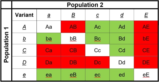
An example of how Dobzhansky-Müller Incompatibilities arise, adapted from Coyne & Orr (2004). We start with an initial population (center top), which splits into two separate populations. In this example, we’ll look at how 5 genes (each letter = one gene) change over time in the separate populations, with the original allele of the gene (lowercase) occasionally mutating into a new allele (upper case). These mutations happen at random times and in random genes in each population (the red letters), such that the two become very different over time. After a while, these two populations might form hybrids; however, given the number of changes in each population, this hybrid might have some combinations of alleles that are ‘untested’ in their evolutionary history (see below). These untested combinations may cause the hybrid to be infertile or unviable, making the two populations isolated species.The list of ‘untested’ genetic combinations from the above example. This table shows the different combinations of each gene that could be made in a hybrid if these two populations interbred. The red cells indicate combinations that have never been ‘tested’ together; that is, at no point in the evolutionary history of these two populations were those two particular alleles together in the same individual. Green cells indicate ones that were together at some point, and thus are expected to be viable combinations (since the resultant populations are obviously alive and breeding).
How can we look at speciation in action?
We can study the process of speciation in the natural world without focussing on the ‘reproductive isolation’ element of species identity as well. For many species, we are unlikely to have the detail (such as an annotated genome and known functions of genes related to reproduction) required to study speciation at this level in any case. Instead, we might choose to focus on the different factors that are currently influencing the process of speciation, such as how the environmental, demographic or adaptive contexts of populations plays a role in the formation of new species. Many of these questions fall within the domain of phylogeography; particularly, how the historical environment has shaped the diversity of populations and species today.
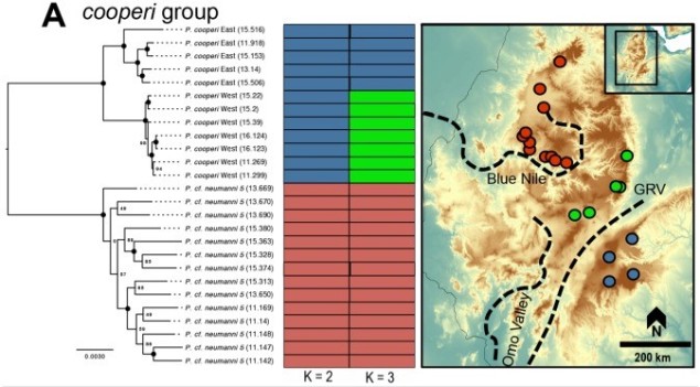
An example of the interplay between speciation and phylogeography, taken from Reyes-Velasco et al. (2018). They investigated the phylogeographic history of several different groups of species within the frog genus Ptychadena; in this figure, we can see how the different species (indicated by the colours and tree on the left) relate to the geography of their habitat (right).
A variety of different analytical techniques can be used to build a picture of the speciation process for closely related or incipient species. A good starting point for any speciation study is to look at how the different study populations are adapting; is there evidence that natural selection is pushing these populations towards different genotypes or ecological niches? If so, then this might be a precursor for speciation, and we can build on this inference with other complementary analyses.
For example, estimating divergence times between populations can help us suggest whether there has been sufficient time for speciation to occur (although this isn’t always clear cut). Additionally, we could estimate the levels of genetic hybridisation (‘introgression’) between two populations to suggest whether they are reasonably isolated and divergent enough to be considered functional species.
The future of speciation genomics
Although these can help answer some questions related to speciation, new tools are constantly needed to provide a clearer picture of the process. Understanding how and why new species are formed is a critical aspect of understanding the world’s biodiversity. How can we predict if a population will speciate at some point? What environmental factors are most important for driving the formation of new species? How stable are species identities, really? These questions (and many more) remain elusive for a wide variety of life on Earth.