We’ve spent some time before discussing the nature of the term ‘species’ and what it means in reality. Of course, answers to questions in biology are always more complicated than we wish they might be, and despite the common nomenclature of the word ‘species’ the underlying definition is convoluted and variable.
Australia is renowned for its unique diversity of species, and likewise for the diversity of ecosystems across the island continent. Although many would typically associate Australia with the golden sandy beaches, palm trees and warm weather of the tropical east coast, other ecosystems also hold both beautiful and interesting characteristics. Even the regions that might typically seem the dullest – the temperate zones in the southern portion of the continent – themselves hold unique stories of the bizarre and wonderful environmental history of Australia.
The two temperate zones
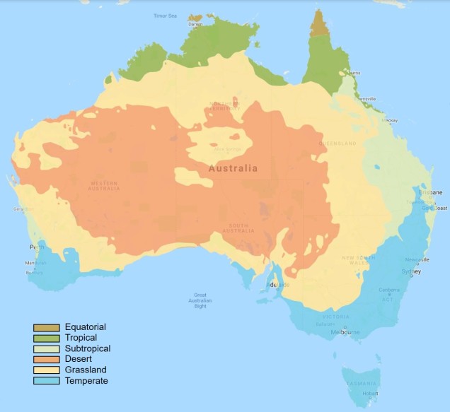
Within Australia, the temperate zone is actually separated into two very distinct and separate regions. In the far south-western corner of the continent is the southwest Western Australia temperate zone, which spans a significant portion. In the southern eastern corner, the unnamed temperate zone spans from the region surrounding Adelaide at its westernmost point, expanding to the east and encompassing Tasmanian and Victoria before shifting northward into NSW. This temperate zones gradually develops into the sub-tropical and tropical climates of more northern latitudes in Queensland and across to Darwin.
The climatic classification (Koppen-Geiger) of Australia’s ecosystems, derived from the Atlas of Living Australia. The light blue region highlights the temperate zones discussed here, with an isolated region in the SW and the broader region of the SE as it transitions into subtropical and tropical climates northward.
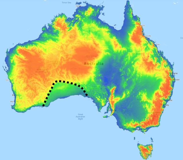
The divide separating these two regions might be familiar to some readers – the Nullarbor Plain. Not just a particularly good location for fossils and mineral ores, the Nullarbor Plain is an almost perfectly flat arid expanse that stretches from the western edge of South Australia to the temperate zone of the southwest. As the name suggests, the plain is totally devoid of any significant forestry, owing to the lack of available water on the surface. This plain is a relatively ancient geological structure, and finished forming somewhere between 14 and 16 million years ago when tectonic uplift pushed a large limestone block upwards to the surface of the crust, forming an effective drain for standing water with the aridification of the continent. Thus, despite being relatively similar bioclimatically, the two temperate zones of Australia have been disconnected for ages and boast very different histories and biota.
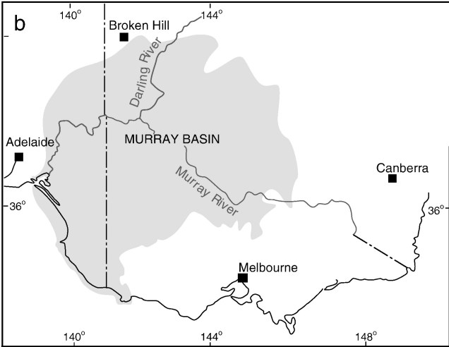
A map of elevation across the Australian continent, also derived from the Atlas of Living Australia. The dashed black line roughly outlines the extent of the Nullarbor Plain, a massively flat arid expanse.
The hotspot of the southwest
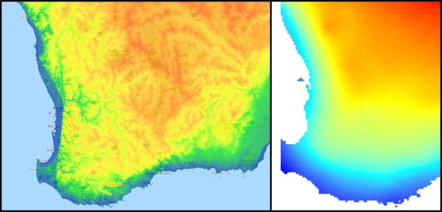
The southwest temperate zone – commonly referred to as southwest Western Australia (SWWA) – is an island-like bioregion. Isolated from the rest of the temperate Australia, it is remarkably geologically simple, with little topographic variation (only the Darling Scarp that separates the lower coast from the higher elevation of the Darling Plateau), generally minor river systems and low levels of soil nutrients. One key factor determining complexity in the SWWA environment is the isolation of high rainfall habitats within the broader temperate region – think of islands with an island.
A figure demonstrating the environmental characteristics of SWWA, using data from the Atlas of Living Australia. Left: An elevation map of the region, showing some mountainous variation, but only one significant steep change along the coast (blue area). Right: A summary of 19 different temperature and precipitation variables, showing a relatively weak gradient as the region shifts inland.
Despite the lack of geological complexity and the perceived diversity of the tropics, the temperate zone of SWWA is the only internationally recognisedbiodiversity hotspot within Australia. As an example, SWWA is inhabited by ~7,000 different plant species, half of which are endemic to the region. Not to discredit the impressive diversity of the rest of the continent, of course. So why does this area have even higher levels of species diversity and endemism than the rest of mainland Australia?
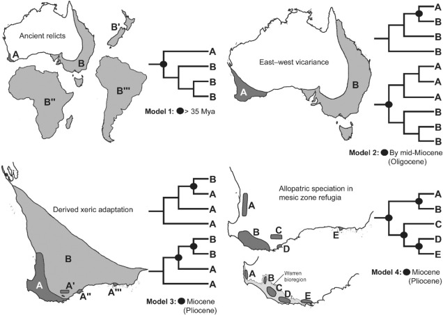
A demonstration of some of the different patterns which might explain the high biodiversity of SWWA, from Rix et al. (2015). These predominantly relate to different biogeographic mechanisms that might have driven diversification in the region, from survivors of the Gondwana era to the more recent fragmentation of mesic habitats.
Well, a number of factors may play significant roles in determining this. One of these is the ancient and isolated nature of the region: SWWA has been separated from the rest of Australia for at least 14 million years, with many species likely originating much earlier than this. Because of this isolation, species occurring within SWWA have been allowed to undergo adaptive divergence from their east coast relatives, forming unique evolutionary lineages. Furthermore, the southwest corner of the continent was one of the last to break away from Antarctica in the dismantling of Gondwana >30 million years ago. Within the region more generally, isolation of mesic (wetter) habitats from the broader, arid (xeric) habitats also likely drove the formation of new species as distributions became fragmented or as species adapted to the new, encroaching xeric habitat. Together, this varies mechanisms all likely contributed in some way to the overall diversity of the region.
The temperate south-east of Australia
Contrastingly, the temperate region in the south-east of the continent is much more complex. For one, the topography of the zone is much more variable: there are a number of prominent mountain chains (such as the extended Great Dividing Range), lowland basins (such as the expansive Murray-Darling Basin) and variable valley and river systems. Similarly, the climate varies significantly within this temperate region, with the more northern parts featuring more subtropical climatic conditions with wetter and hotter summers than the southern end. There is also a general trend of increasing rainfall and lower temperatures along the highlands of the southeast portion of the region, and dry, semi-arid conditions in the western lowland region.
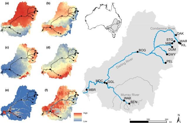
A map demonstrating the climatic variability across the Murray-Darling Basin (which makes up a large section of the SE temperate zone), from Brauer et al. (2018). The different heat maps on the left describe different types of variables; a) and b) represent temperature variables, c) and d) represent precipitation (rainfall) variables, and e) and f) represent water flow variables. Each variable is a summary of a different set of variables, hence the differences.
A complicated history
The south-east temperate zone is not only variable now, but has undergone some drastic environmental changes over history. Massive shifts in geology, climate and sea-levels have particularly altered the nature of the area. Even volcanic events have been present at some time in the past.
One key hydrological shift that massively altered the region was the paleo-megalake Bungunnia. Not just a list of adjectives, Bungunnia was exactly as it’s described: a historically massive lake that spread across a huge area prior to its demise ~1-2 million years ago. At its largest size, Lake Bungunnia reached an area of over 50,000 km2, spreading from its westernmost point near the current Murray mouth although to halfway across Victoria. Initially forming due to a tectonic uplift event along the coastal edge of the Murray-Darling Basin ~3.2 million years ago, damming the ancestral Murray River (which historically outlet into the ocean much further east than today). Over the next few million years, the size of the lake fluctuated significantly with climatic conditions, with wetter periods causing the lake to overfill and burst its bank. With every burst, the lake shrank in size, until a final break ~700,000 years ago when the ‘dam’ broke and the full lake drained.
A map demonstrating the sheer size of paleo megalake Bungunnia at it’s largest extent, taken from McLaren et al. (2012).
Another change in the historic environment readers may be more familiar with is the land-bridge that used to connect Tasmania to the mainland. Dubbed the Bassian Isthmus, this land-bridge appeared at various points in history of reduced sea-levels (i.e. during glacial periods in Pleistocene cycle), predominantly connecting via the still-above-water Flinders and Cape Barren Islands. However, at lower sea-levels, the land bridge spread as far west as King Island: central to this block of land was a large lake dubbed the Bass Lake (creative). The Bassian Isthmus played a critical role in the migration of many of the native fauna of Tasmania (likely including the Indigenous peoples of the now-island), and its submergence and isolation leads to some distinctive differences between Tasmanian and mainland biota. Today, the historic presence of the Bassian Isthmus has left a distinctive mark on the genetic make-up of many species native to the southeast of Australia, including dolphins, frogs, freshwater fishes and invertebrates.
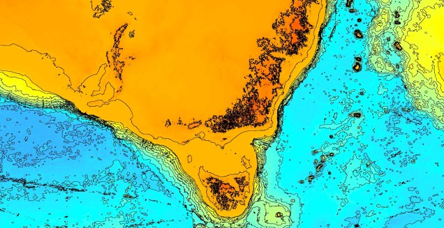
An elevation (Etopo1) map demonstrating the now-underwater land bridge between Tasmania and the mainland. Orange colours denote higher areas whilst light blue represents lower sections.
Don’t underestimate the temperates
Although tropical regions get most of the hype for being hotspots of biodiversity, the temperate zones of Australia similarly boast high diversity, unique species and document a complex environmental history. Studying how the biota and environment of the temperate regions has changed over millennia is critical to predicting the future effects of climatic change across large ecosystems.
To expand on this, we’re going to look at a few different models of how the spatial distribution of populations influences their divergence, and particularly how these factor into different processes of speciation.
What comes first, ecological or genetic divergence?
The order of these two processes have been in debate for some time, and different aspects of species and the environment can influence how (or if) these processes occur.
Different spatial models of speciation
Generally, when we consider the spatial models for speciation we divide these into distinct categories based on the physical distance of populations from one another. Although there is naturally a lot of grey area (as there is with almost everything in biological science), these broad concepts help us to define and determine how speciation is occurring in the wild.
The standard model of allopatric speciation, following an island model. 1) We start with a single population occupying a single island. 2) A rare dispersal event pushes some individuals onto a new island, forming a second population. Note that this doesn’t happen often enough to allow for consistent gene flow (i.e. the island was only colonised once). 3) Over time, these populations may accumulate independent genetic and ecological changes due to both natural selection and drift, and when they become so different that they are reproductively isolated they can be considered separate species.
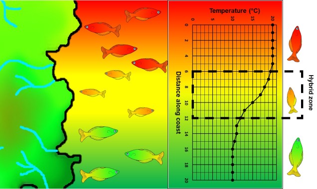
A step closer in bringing populations geographically together in speciation is “parapatry” and “peripatry”. Parapatric populations are often geographically close together but not overlapping: generally, the edges of their distributions are touching but do not overlap one another. A good analogy would be to think of countries that share a common border. Parapatry can occur when a species is distributed across a broad area, but some form of narrow barrier cleaves the distribution in two: this can be the case across particular environmental gradients where two extremes are preferred over the middle.
An example of parapatric species across an environment gradient (in this case, a temperature gradient along the ocean coastline). Left: We have two main species (red and green fish) which are adapted to either hotter or colder temperatures (red and green in the gradient), respectively. A small zone of overlap exists where hybrid fish (yellow) occur due to intermediate temperature. Right: How the temperature varies across the system, forming a steep gradient between hot and cold waters.
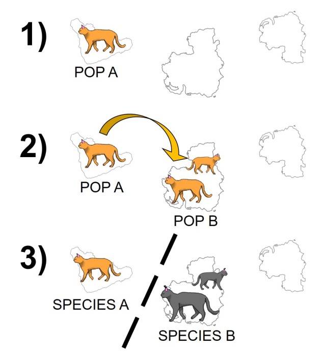
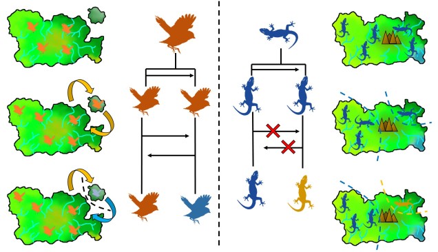
The two main ways peripatric species can form. Left: The dispersal method. In this example, there is a central ‘source’ population (orange birds on the main island), which holds most of the distribution. However, occasionally (more frequently than in the allopatric example above) birds can disperse over to the smaller island, forming a (mostly) independent secondary population. If the gene flow between this population and the central population doesn’t overwhelm the divergence between the two populations (due to selection and drift), then a new species (blue birds) can form despite the gene flow. Right: The range contraction method. In this example, we start with a single widespread population (blue lizards) which has a rapid reduction in its range. However, during this contraction one population is separated from the main body (i.e. as a refugia), which may also be a precursor of peripatric speciation.
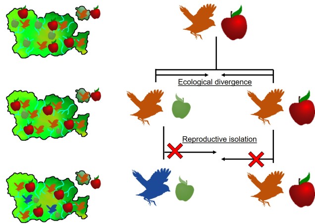
This can be tricky to visualise, so let’s invent an example. Say we have a tropical island, which is occupied by one bird species. This bird prefers to eat the large native fruit of the island, although there is another fruit tree which produces smaller fruits. However, there’s only so much space and eventually there are too many birds for the number of large fruit trees available. So, some birds are pushed to eat the smaller fruit, and adapt to a different diet, changing physiology over time to better acquire their new food and obtain nutrients. This shift in ecological niche causes the two populations to become genetically separated as small-fruit-eating-birds interact more with other small-fruit-eating-birds than large-fruit-eating-birds. Over time, these divergences in genetics and ecology causes the two populations to form reproductively isolated species despite occupying the same island.
A diagram of the ecological speciation example given above. Note that ecological divergence occurs first, with some birds of the original species shifting to the new food source (‘ecological niche’) which then leads to speciation. An important requirement for this is that gene flow is somehow (even if not totally) impeded by the ecological divergence: this could be due to birds preferring to mate exclusively with other birds that share the same food type; different breeding seasons associated with food resources; or other isolating mechanisms.
As you can see, the processes and context driving speciation are complex to unravel and many factors play a role in the transition from population to species. Understanding the factors that drive the formation of new species is critical to understanding not just how evolution works, but also in how new diversity is generated and maintained across the globe (and how that might change in the future).
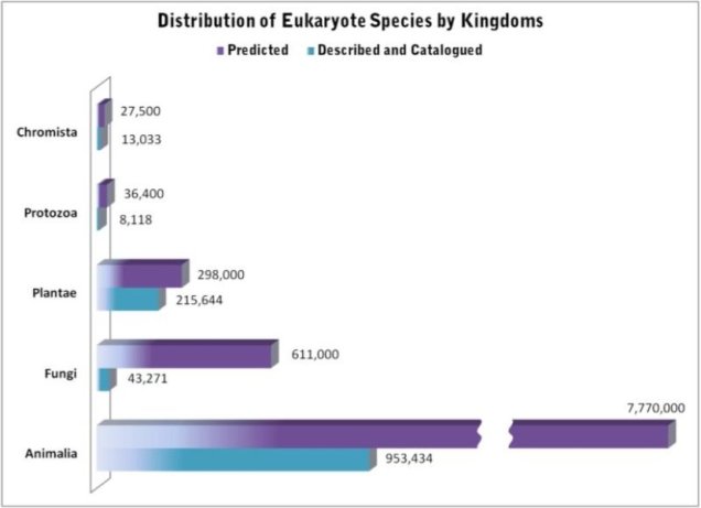
There are quite literally millions of species on Earth, ranging from the smallest of microbes to the largest of mammals. In fact, there are so many that we don’t actually have a good count on the sheer number of species and can only estimate it based on the species we actually know about. Unsurprisingly, then, the number of species vastly outweighs the number of people that research them, especially considering the sheer volumes of different aspects of species, evolution, conservation and their changes we could possibly study.
Some estimations on the number of eukaryotic species (i.e. not including things like bacteria), with the number of known species in blue and the predicted number of total species on Earth in purple. Source: Census of Marine Life.
This is partly where the concept of a ‘model’ comes into it: it’s much easier to pick a particular species to study as a target, and use the information from it to apply to other scenarios. Most people would be familiar with the concept based on medical research: the ‘lab rat’ (or mouse). The common house mouse (Mus musculus) and the brown rat (Rattus norvegicus) are some of the most widely used models for understanding the impact of particular biochemical compounds on physiology and are often used as the testing phase of medical developments before human trials.
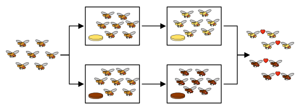
A simplified summary of the speciation experiment in Drosophila, starting with a single species and resulting in two reproductively isolated species based on mating and food preference. Source: Ilmari Karonen, adapted from here.
Some of Darwin’s early drawings of the morphological differences in Galapagos finch beaks, which lead to the formulation of the theory of evolution by natural selection.
The sheer diversity of species and form makes African cichlids an ideal model for testing hypotheses and theories about the process of evolution and adaptive radiation. Figure sourced from Brawand et al. (2014) in Nature.
This is the fourth (and final) part of the miniseries on the genetics and process of speciation. To start from Part One, click here.
In last week’s post, we looked at how we can use genetic tools to understand and study the process of speciation, and particularly the transition from populations to species along the speciation continuum. Following on from that, the question of “how many species do I have?” can be further examined using genetic data. Sometimes, it’s entirely necessary to look at this question using genetics (and genomics).
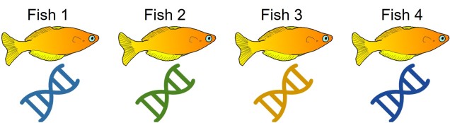
An example of cryptic species. All four fish in this figure are morphologically identical to one another, but they differ in their underlying genetic variation (indicated by the different colours of DNA). Thus, from looking at these fish alone we would not perceive any differences, but their genetic make-up might suggest that there are more than one species…The level of genetic differentiation between the fish in the above example. The phylogenies on the left and top of the figure demonstrate the evolutionary relationships of these four fish. The matrix shows a heatmap of the level of differences between different pairwise comparisons of all four fish: red squares indicate zero genetic differences (such as when comparing a fish to itself; the middle diagonal) whilst yellow squares indicate increasingly higher levels of genetic differentiation (with bright yellow = all differences). By comparing the different fish together, we can see that Fish 1 and 2, and Fish 3 and 4, are relatively genetically similar to one another (red-deep orange). However, other comparisons show high level of genetic differences (e.g. 1 vs 3 and 1 vs 4). Based on this information, we might suggest that Fish 1 and 2 belong to one cryptic species (A) and Fish 3 and 4 belong to a second cryptic species (B).
Genetic tools to study species: the ‘Barcode of Life’
A classically employed method that uses DNA to detect and determine species is referred to as the ‘Barcode of Life’. This uses a very specific fragment of DNA from the mitochondria of the cell: the cytochrome c oxidase I gene, CO1. This gene is made of 648 base pairs and is found pretty well universally: this and the fact that CO1 evolves very slowly make it an ideal candidate for easily testing the identity of new species. Additionally, mitochondrial DNA tends to be a bit more resilient than its nuclear counterpart; thus, small or degraded tissue samples can still be sequenced for CO1, making it amenable to wildlife forensics cases. Generally, two sequences will be considered as belonging to different species if they are certain percentage different from one another.
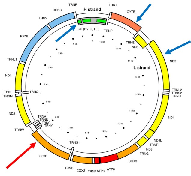
The full (annotated) mitochondrial genome of humans, with the different genes within it labelled. The CO1 gene is labelled with the red arrow (sometimes also referred to as COX1) whilst blue arrows point to other genes often used in phylogenetic or taxonomic studies, depending on the group or species in question.
Despite the apparent benefits of CO1, there are of course a few drawbacks. Most of these revolve around the mitochondrial genome itself. Because mitochondria are passed on from mother to offspring (and not at all from the father), it reflects the genetic history of only one sex of the species. Secondly, the actual cut-off for species using CO1 barcoding is highly contentious and possibly not as universal as previously suggested. Levels of sequence divergence of CO1 between species that have been previously determined to be separate (through other means) have varied from anywhere between 2% to 12%. The actual translation of CO1 sequence divergence and species identity is not all that clear.
Gene tree – species tree incongruences
One particularly confounding aspect of defining species based on a single gene, and with using phylogenetic-based methods, is that the history of that gene might not actually be reflective of the history of the species. This can be a little confusing to think about but essentially leads to what we call “gene tree – species tree incongruence”. Different evolutionary events cause different effects on the underlying genetic diversity of a species (or group of species): while these may be predictable from the genetic sequence, different parts of the genome might not be as equally affected by the same exact process.
A classic example of this is hybridisation. If we have two initial species, which then hybridise with one another, we expect our resultant hybrids to be approximately made of 50% Species A DNA and 50% Species B DNA (if this is the first generation of hybrids formed; it gets a little more complicated further down the track). This means that, within the DNA sequence of the hybrid, 50% of it will reflect the history of Species A and the other 50% will reflect the history of Species B, which could differ dramatically. If we randomly sample a single gene in the hybrid, we will have no idea if that gene belongs to the genealogy of Species A or Species B, and thus we might make incorrect inferences about the history of the hybrid species.
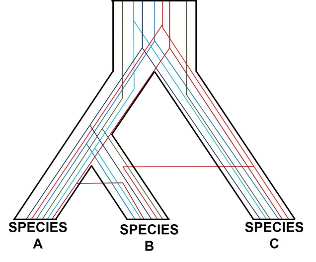
A diagram of gene tree – species tree incongruence. Each individual coloured line represents a single gene as we trace it back through time; these are mostly bound within the limits of species divergences (the black borders). For many genes (such as the blue ones), the genes resemble the pattern of species divergences very well, albeit with some minor differences in how long ago the splits happened (at the top of the branches). However, the red genes contrast with this pattern, with clear movement across species (from A and C into B): this represents genes that have been transferred by hybridisation. The green line represents a gene affected by what we call incomplete lineage sorting; that is, we cannot trace it back far enough to determine exactly how/when it initially diverged and so there are still two separate green lines at the very top of the figure. You can think of each line as a separate phylogenetic tree, with the overarching species tree as the average pattern of all of the genes.
There are a number of other processes that could similarly alter our interpretations of evolutionary history based on analysing the genetic make-up of the species. The best way to handle this is simply to sample more genes: this way, the effect of variation of evolutionary history in individual genes is likely to be overpowered by the average over the entire gene pool. We interpret this as a set of individual gene trees contained within a species tree: although one gene might vary from another, the overall picture is clearer when considering all genes together.
Species delimitation
In earlier posts on The G-CAT, I’ve discussed the biogeographical patterns unveiled by my Honours research. Another key component of that paper involved using statistical modelling to determine whether cryptic species were present within the pygmy perches. I didn’t exactly elaborate on that in that section (mostly for simplicity), but this type of analysis is referred to as ‘species delimitation’. To try and simplify complicated analyses, species delimitation methods evaluate possible numbers and combinations of species within a particular dataset and provides a statistical value for which configuration of species is most supported. One program that employs species delimitation is Bayesian Phylogenetics and Phylogeography(BPP): to do this, it uses a plethora of information from the genetics of the individuals within the dataset. These include how long ago the different populations/species separated; which populations/species are most related to one another; and a pre-set minimum number of species (BPP will try to combine these in estimations, but not split them due to computational restraints). This all sounds very complex (and to a degree it is), but this allows the program to give you a statistical value for what is a species and what isn’t based on the genetics and statistical modelling.
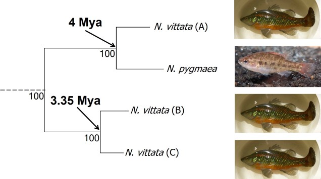
The cryptic species of pygmy perches identified within my research paper. This represents part of the main phylogenetic tree result, with the estimates of divergence times from other analyses included. The pictures indicate the physiology of the different ‘species’: Nannoperca pygmaea is morphologically different to the other species of Nannoperca vittata. Species delimitation analysis suggested all four of these were genetically independent species; at the very least, it is clear that there must be at least 2 species of Nannoperca vittata since A is more related to N. pygmaea than to other N. vittata species. Photo credits: N. vittata = Chris Lamin; N. pygmaea = David Morgan.
The end result of a BPP run is usually reported as a species tree (e.g. a phylogenetic tree describing species relationships) and statistical support for the delimitation of species (0-1 for each species). Because of the way the statistical component of BPP works, it has been found to give extremely high support for species identities. This has been criticised as BPP can, at time, provide high statistical support for genetically isolated lineages (i.e. divergent populations) which are not actually species.
Improving species identities with integrative taxonomy
Due to this particular drawback, and the often complex nature of species identity, using solely genetic information such as species delimitation to define species is extremely rare. Instead, we use a combination of different analytical techniques which can include genetic-based evaluations to more robustly assign and describe species. In my own paper example, we suggested that up to three ‘species’ of N. vittata that were determined as cryptic species by BPP could potentially exist pending on further analyses. We did not describe or name any of the species, as this would require a deeper delve into the exact nature and identity of these species.
As genetic data and analytical techniques improve into the future, it seems likely that our ability to detect and determine species boundaries will also improve. However, the additional supported provided by alternative aspects such as ecology, behaviour and morphology will undoubtedly be useful in the progress of taxonomy.