Bigger and better: the evolution of genomic markers

From genetic to genomic markers

As we discussed in last week’s post, different parts of the DNA can be used as genetic markers for analyses relating to conservation, ecology and evolution. We looked at a few different types of markers (allozymes, microsatellites, mitochondrial DNA) and why different markers are good for different things. This week, we’ll focus on the much grander and more modern state of genomics; that is, using DNA markers that are often thousands of genes big!

Genomics vs genetics — If we pretended that the size of the text for each marker was indicative of how big the data is, this figure would probably be about a 1000x under-estimation of genomic datasets. There is not enough room on the blog page to actually capture this.

I briefly mentioned last week that the development of genomics was largely facilitated by what we call ‘next-generation sequencing’, which allows us to easily obtain billions of fragments of DNA and collate them into a useful dataset. Most genomic technologies differ based on how they fragment the DNA for sequencing and how the data is processed.

While the analytical, monetary and time cost of obtaining genomic data has decreased as sequencing technology has improved, we still need to balance these factors together when deciding which method to use. Many methods allow us to put many individual samples together in the same reaction (we tell which sequence belongs to which sequence using special ‘barcode sequences’ that code for one specific sample): in this case, we also need to consider how many samples to place together (“multiplex”).

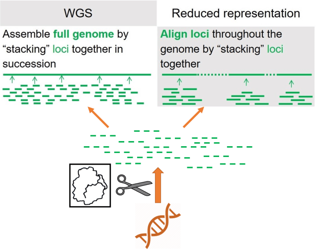
As a broad generalisation, we can separate most genomic sequencing methods into two broad categories: whole genome or reduced-representation. As the name suggests, whole genome sequencing involves collecting the entire genome of the individuals we use, although this is generally very expensive and can only be done with a limited number of samples at a time. If we want to have a much larger dataset, often we’ll use reduced-representation methods: these involve breaking down the whole genome into much smaller fragments and as many of these as we can to get a broad overview of the genome. Reduced-representation methods are much cheaper and are appropriate for larger sample sizes than whole genome, but naturally lose large amounts of information from the genome.

Genomic sequencing pathway — The (very, very) vague outline of genomic sequencing. First we take all of the DNA of an organism, breaking it into smaller fragments in this case using a restriction enzyme (see below). We then amplify these fragments, making billions of copies of them before piecing them back together to either make the entire genome (left) of a few individuals or patches of the genome (right) for more individuals.

Restriction-site associated DNA (RADseq)

Within the Molecular Ecology Lab, we predominantly use a technology known as “double digest restriction site-associated DNA sequencing”, which is a huge mouthful so we just call it ‘ddRAD’. This sounds incredibly complicated, but (as far as sequencing methods go, anyway) is actually relatively simple. We take the genome of a sample, and then using particular enzymes (called ‘restriction enzymes’), we break the genome randomly down into small fragments (usually up to 200 bases long, after we filter it). We then attach a specific barcode for that individual, and a few more bits and pieces as part of the sequencing process, and then pool them together. This pool (a “library”) is sent off to a facility to be run through a sequencing machine and produce the data we work with. The ‘dd’ part of ‘ddRAD’ just means that a pair of restriction enzymes are used in this method, instead of just one (it’s a lot cleaner and more efficient).

ddRAD flowchart — A simplified standard ddRAD protocol. 1) We obtain the DNA-containing tissue of the organism we want to study, such as blood, skin or muscle samples. 2) We extract all of the genomic DNA from the tissue sample, making sure we have good quantity and quality (avoiding degradation if possible). 3) We break the genome down into smaller fragments using restriction enzymes, which cut at certain places (orange and green marks on the top line). We then attach special sequences to these fragments, such as the adapter (needed for the sequencer to work) and the barcode for that specific individual organism (the green bar). 4) We amplify the fragments, generating billions of copies of each of them. 5) We send these off to a sequencing facility to read the DNA sequence of these fragments (often outsourced to a private institution). 6) We get back a massive file containing all of the different sequences for all of the organisms in one file. 7) We separate out these sequences into the individual the came from by using their special barcode as an identifier (the coloured codes). 8) We then process this data to make sure it’s of the best quality possible, including removing sequences that we don’t have enough copies of or have errors. From this, we produce a final dataset, often with one continuous sequence for each individual. If this dataset doesn’t meet our standards for quality or quantity, we go back and try new filtering parameters.

Gene expression and transcriptomics

Sometimes, however, we might not even want to look at the exact DNA sequence. You might remember in an earlier blog post that I mentioned genes can be ‘switched on’ or ‘switched off’ by activator or repressor proteins. Well, because of this, we can have the exact same genes act in different ways depending on the environment. This is most observable in tissue development: although all of the cells of all of your organs have the exact same genome, the control of gene expression changes what genes are active and thus the physiology of the organ. We might also have genes which are only active in an organism under certain conditions, like heat shock proteins under hot conditions.

This can be an important part of evolution as being able to easily change genetic expression may allow an individual to adapt to new environmental pressures much more easily; we call this ‘phenotypic plasticity’. In this case, instead of sequencing the DNA, we might want to look at which genes are expressed, or how much they are expressed, in different conditions or populations: this is called ‘comparative transcriptomics’. So instead of sequencing the DNA, we sequence the RNA of an organism (the middle step of making proteins, so most RNAs are only present if the gene is being expressed).

Processing data

Despite how it must appear, most of the work with genomic datasets actually comes after you get the sequences back. Because of the nature and scale of genomic datasets, rigorous analytical pipelines are needed to manage and filter data from the billions of small sequences into full sequences of high quality. There are many different ways to do this, and usually involves playing with parameters, so I won’t delve into the details (although some of it is explained in the boxed part of the flowchart figure).

The future of genomics

No doubt as the technology improves, whole genome sequencing will become progressively more feasible for more species, opening up the doors for a new avalanche of data and possibilities. In any case, we’ve come a long way since the first whole genome (for Haemophilus influenzae) in 1995 and the construction of the whole human genome in 2003.