The nature of adaptation
One of the most fundamental aspects of natural selection and evolution is, of course, the underlying genetic traits that shape the physical, selected traits. Most commonly, this involves trying to understand how changes in the distribution and frequencies of particular genetic variants (alleles) occur in nature and what forces of natural election are shaping them. Remember that natural selection acts directly on the physical characteristics of species; if these characteristics are genetically-determined (which many are), then we can observe the flow-on effects on the genetic diversity of the target species.
Although we might expect that natural selection is a fairly predictable force, there are a myriad of ways it can shape, reduce or maintain genetic diversity and identity of populations and species. In the following examples, we’re going to assume that the mentioned traits are coded for by a single gene with two different alleles for simplicity. Thus, one allele = one version of the trait (and can be used interchangeably). With that in mind, let’s take a look at the three main broad types of changes we observe in nature.
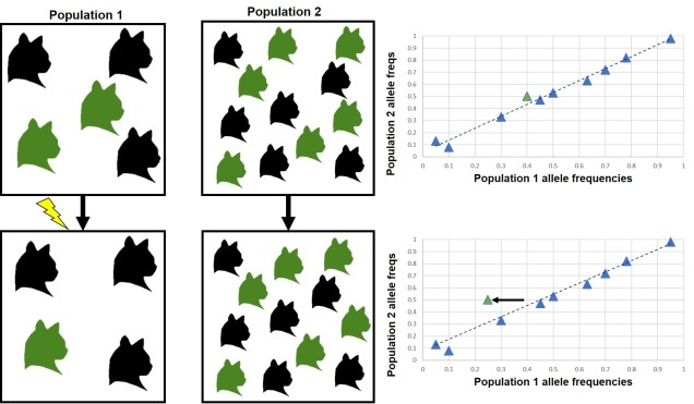
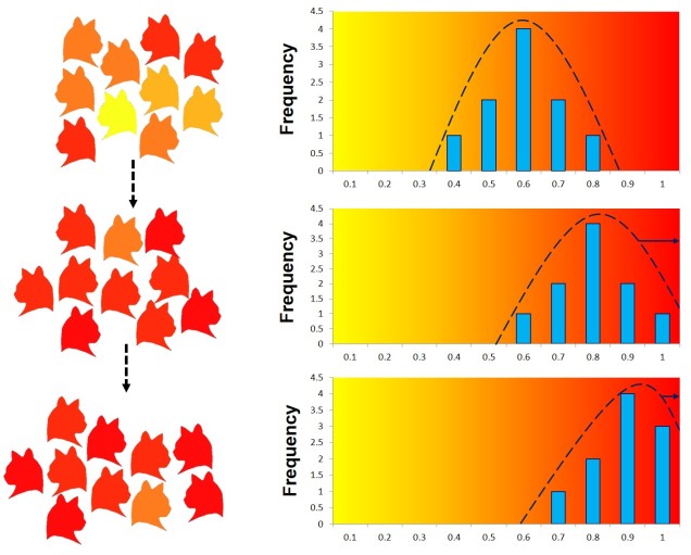
Directional selection
Arguably the most traditional perspective of natural selection is referred to as ‘directional selection’. In this example, nature selection causes one allele to be favoured more than another, which causes it to increase dramatically in frequency compared to the alternative allele. The reverse effect (natural selection pushing against a maladaptive allele) is still covered by directional selection, except that it functions in the opposite way (the allele under negative selection has reduced frequency, shifting towards the alternative allele).
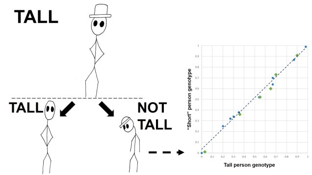
Balancing selection
Natural selection doesn’t always push allele frequencies into different directions however, and sometimes maintains the diversity of alleles in the population. This is what happens in ‘balancing selection’ (sometimes also referred to as ‘stabilising selection’). In this example, natural selection favours non-extreme allele frequencies, and pushes the distribution of allele frequencies more to the centre. This may happen if deviations from the original gene, regardless of the specific change, can have strongly negative effects on the fitness of an organism, or in genes that are most fit when there is a decent amount of variation within them in the population (such as the MHC region, which contributes to immune response). There are a couple other reasons balancing selection may occur, though.
Heterozygote advantage
One example is known as ‘heterozygote advantage’. This is when an organism with two different alleles of a particular gene has greater fitness than an organism with two identical copies of either allele. A seemingly bizarre example of heterozygote advantage is related to sickle cell anaemia in African people. Sickle cell anaemia is a serious genetic disorder which is encoded for by recessive alleles of a haemoglobin gene; thus, a person has to carry two copies of the disease allele to show damaging symptoms. While this trait would ordinarily be strongly selected against in many population, it is maintained in some African populations by the presence of malaria. This seems counterintuitive; why does the presence of one disease maintain another?
Well, it turns out that malaria is not very good at infecting sickle cells; there are a few suggested mechanisms for why but no clear single answer. Naturally, suffering from either sickle cell anaemia or malaria is unlikely to convey fitness benefits. In this circumstance, natural selection actually favours having one sickle cell anaemia allele; while being a carrier isn’t ordinarily as healthy as having no sickle cell alleles, it does actually make the person somewhat resistant to malaria. Thus, in populations where there is a selective pressure from malaria, there is a heterozygote advantage for sickle cell anaemia. For those African populations without likely exposure to malaria, sickle cell anaemia is strongly selected against and less prevalent.

Frequency-dependent selection
Another form of balancing selection is called ‘frequency-dependent selection’, where the fitness of an allele is inversely proportional to its frequency. Thus, once the allele has become common due to selection, the fitness of that allele is reduced and selection will start to favour the alternative allele (which is at much lower frequency). The constant back-and-forth tipping of the selective scales results in both alleles being maintained at an equilibrium.
This can happen in a number of different ways, but often the rarer trait/allele is fundamentally more fit because of its rarity. For example, if one allele allows an individual to use a new food source, it will be very selectively fit due to the lack of competition with others. However, as that allele accumulates within the population and more individuals start to feed on that food source, the lack of ‘uniqueness’ will mean that it’s not particularly better than the original food source. A balance between the two food sources (and thus alleles) will be maintained over time as shifts towards one will make the other more fit, and natural selection will compensate.

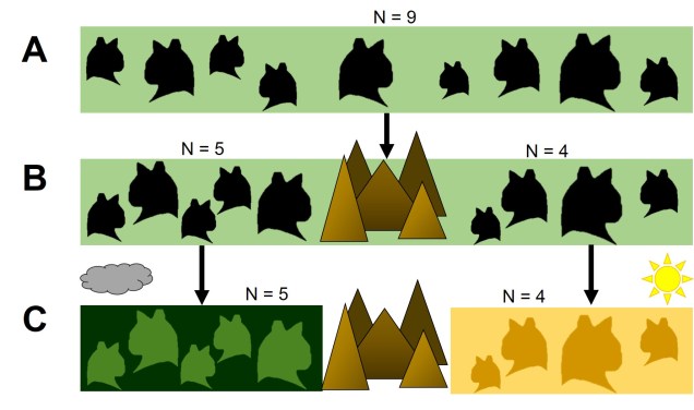
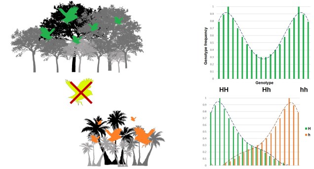
Disruptive selection
A third category of selection (although not as frequently mentioned) is known as ‘disruptive selection’, which is essentially the direct opposite of balancing selection. In this case, both extremes of allele frequencies are favoured (e.g. 1 for one allele or 1 for the other) but intermediate frequencies are not. This can be difficult to untangle in natural populations since it could technically be attributed to two different cases of directional selection. Each allele of the same gene is directionally selected for, but in opposite populations and directions so that overall pattern shows very little intermediates.
In direct contrast to balancing selection, disruptive selection can often be a case of heterozygote disadvantage (although it’s rarely called that). In these examples, it may be that individuals which are not genetically committed to one end or the other of the frequency spectrum are maladapted since they don’t fit in anywhere. An example would be a species that occupies both the desert and a forested area, with little grassland-type habitat in the middle. For the relevant traits, strongly desert-adapted genes would be selected for in the desert and strongly forest-adapted genes would be selected for in the forest. However, the lack of gradient between the two habitats means that individuals that are half-and-half are less adaptive in both the desert and the forest. A case of jack-of-all-trades, master of none.
Direction of selection
Although it would be convenient if natural selection was entirely predictable, it often catches up by surprise in how it acts and changes species and populations in the wild. Careful analysis and understanding of the different processes and outcomes of adaptation can feed our overall understanding of evolution, and aid in at least pointing in the right direction for our predictions.