Genomics

Origination of adaptation: the old and the new (genes)

September 1, 2018Sean Buckley3 Comments

Adaptation is arguably the most critical biological process in the evolution of species. The process of evolution by natural selection is the cornerstone of evolutionary biology (and indeed, all of contemporary biology!) and adaptation remains fundamental to the process. We know that adaptation is based on the idea that some genetic variants are ‘better’ adapted than others, and thus are unequally shared across a population. But where does this genetic variation come from?

The accumulation of new genetic variation

The classic way for new genetic variants to appear is often thought of as mutation: changes in a single base in the DNA are caused by various external processes such as chemical, physical or environmental influences (such as the sci-fi classics like UV rays or toxic chemicals). Although these forms of mutations happen very rarely and certainly don’t have the same effects comic books would leave you to believe, new mutations can occur relatively rapidly depending on the characteristics of the species. However, the most common way for new mutations to occur is actually part of the DNA replication process: copying DNA is not always perfect and even though the relevant proteins essentially run a spellcheck, sometimes the copy is not 100% perfect and new mutations occur.

Adaptation of mutation figure — An example of how adaptation can occur from a new mutation. In this example, we have one gene (TTXTT), with initial only one allele (variant), TTATT. In the second generation (row), a mutation occurs in one individual which creates a new, second allele: TTGTT. This allele is favoured over the TTATT allele, and in the next generation it’s frequency increases as the alternative allele frequency decreases (the pattern is shown in the frequency values on the right side).

It is important to remember that only mutations that are present in the reproductive cells (sperm and eggs) can be inherited and passed on, and thus be a source for adaptation. Mutations in other tissues of the body, such as within the skin, are not spread across the entire body of the subject and thus aren’t passed on to offspring.

Standing genetic variation

Alternatively, genetic variation might already be present within a species or population. This is more likely if population sizes are large and populations are well connected and interbreeding. We refer to this diverse initial gene pool as ‘standing genetic variation’: that is, the amount of genetic variation within the population or species before the selective pressure requiring adaptation. Standing genetic variation can be thought of as the ‘diversity of choices’ for natural selection to act upon: the variants are readily available, and if a good choice exists it will be favoured by natural selection and become more widespread within the population or species (i.e. evolve).

Adaptation of standing variation figure.jpg — A slightly more complex example of how adaptation can occur from standing variation, this time with two different genes. One codes for fur colour, with two different alleles: GCATA codes for orange fur, and GCGTA codes for grey fur. The other gene codes for ear tufts, with TTCCT coding for tufts and TCCCT coding for no tufts. Natural selection favours both orange fur and tufted ears, and cats with these traits reproduce more frequently than those without (see graph below). These cats probably look familiar.

Graph of standing variation.jpg — The frequency of all four alleles (i.e. either allele for both genes) over the generations in the above figure. Clearly, we can see how adaptation rapidly favours orange fur and tufted ears over grey fur and non-tufted ears with the shifts in frequencies over the different alleles.

We’ve discussed standing genetic variation before on The G-CAT, but often in a different light (and phrasing). For example, when we’ve talked about founder effect: that is, when a population is formed from only a few different individuals which causes it to be very genetically depauperate. In populations under strong founder effect, there is very little standing genetic variation for natural selection to act upon. This has long been an enigma for many pest species: how have they managed to proliferate so widely when they often originate from so few individuals and lack genetic diversity?

Adaptive variation

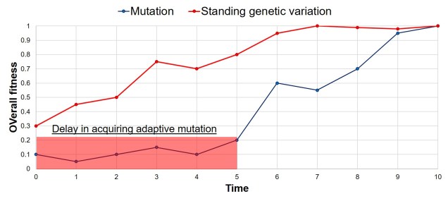
Adaptation may not require new genetic variants to be generated from mutation. If there are a large number of alleles within the gene pool to start with, then natural selection may favour one of those variants over others and allow adaptation to start immediately. Compared to the rate at which new mutations occur, are potentially corrected for in DNA repair, are potentially erased by genetic drift, and then put under selective pressure, adaptation from standing genetic variation can occur very quickly.

Rate of adaptation figure.jpg — A rough example of the speed of adaptation depending on how the adaptive allele originated: whether it was already present (in the form of standing variation), or whether it was created by a new mutation. As one would expect, there is a significant lag delay in adaptation in the mutation scenario, based on the time it takes for said adaptive mutation to be created through relatively random processes. Thus, a positively selected allele from standing variation can allow a species to adapt much faster than waiting for a positive mutation to occur.

Conserving genetic variation

Given the adaptive potential provided by maintaining a good amount of standing genetic variation, it is imperative to conserve genetic diversity within populations in conservation efforts. This is why we often equate genetic diversity with ‘adaptive potential’ of species, although the exact amount of genetic diversity required for adaptive potential depends on a large number of other factors. Clearly, in some instances species show the ability to adapt to new pressures or novel environments even without a large amount of standing genetic variation.

It is important to remember that standing genetic variation consists of two types: neutral genetic diversity, which is not necessarily under selection at the time, and adaptive genetic diversity, which is directly under selection (although this can be either for or against the given variant). However, currently neutral genetic variants may become adaptive variants in the future if selective pressures change: although those different variants aren’t necessarily beneficial or detrimental at the moment, that may change in the future. Thus, conserving both types of genetic diversity is important for the survivability and longevity of populations under conservation programs.

Other types of adaptation

Although genetic diversity is clearly critically important for adaptive potential, alternative mechanisms for adaptation also exist. One of these relies less on the actual genetic variants being different, but rather how individual genes are used. This can happen in a few different ways, but mostly commonly this is through alternative splicing: when a gene is being ‘read’ and a protein is produced, different parts of the gene can be used (and in different order) to make a completely different protein.

Alternate splicing figure.jpg — An extreme example of alternate splicing of one gene. We start with a single gene, composed of 5 (A–E) main gene elements (exons). Different environmental pressures (like fire risk, flooding, cold weather or predators, for example) cause the organism to use different combinations of these exons to make different proteins (right side; A–D). Actual alternate splicing is not usually this straight-forward (one gene doesn’t conveniently split into four forms depending on the threat), but the process is generally the same.

Believe it or not, we’ve sort of discussed the effects of alternative splicing before. Phenotypic plasticity occurs when a single organism can have very different physiological traits depending on the environment: even though the genes are the same, they are utilised in different ways to make a different body shape. This is how some species can look incredibly different when they live in different places even if they’re genetically very similar. That said, for the vast majority of species maintaining good levels of genetic diversity is critical for the survivability of said species.

It takes (at least) two: coevoultion and species interactions

August 24, 2018August 24, 2018Sean Buckley1 Comment

The environmental context of adaptation

We’ve talked many times before about how species evolve in response to some kind of environmental pressure, which favours (or disfavours) certain traits within that species. Over time, this drives changes in the frequencies of species traits and alters the overall average phenotype of that species (sometimes slowly, sometimes rapidly).

While we usually talk about the environment in terms of abiotic conditions such as temperature or climate, biotic factors are equally important: that is, the parts of the environment which are themselves also alive. Because of this, changes in one species can have profound repercussions on other species linked within the ecosystem. Thus, the evolution of one species is intrinsically linked to the evolution of other relevant species within the ecosystem: often, these connected evolutionary pathways battle with one another as each one changes. Let’s take a look at a few different examples of how evolution of one species may impact the evolution of another.

Predator-prey coevolution

One of the most obvious ways the evolution of two different species can interact is in predator and prey relationships. Naturally, prey species evolve to be able to defend themselves from predators in various ways, such as crypsis (e.g. camouflage), toxicity or behavioural changes (such as nocturnalism or group herding). Contrastingly, predators will evolve new and improved methods for detecting and hunting prey, such as enhanced senses, venom and stealth (through soft-padded feet, for example).

There are millions of possible examples of predator-prey coevolution that could be used as examples here, based on the continual drive for one species to get the upper hand over the other. But one that comes to mind is of a creature that I learnt about while on holiday in Scandinavia: the pine marten, and how it affects squirrels.

This photo is one that I took whilst on a lunch break at a bakery in the Norwegian mountains, of a small critter running among the rocks by the lakeside. Not sure exactly what species it was, I asked the tour director who excitedly told me that it was a pine marten. After doing a bit of research on them (and trying to figure out what the difference between a pine marten, a stoat, and a weasel is), I’ve discovered that it’s actually more likely to be a stoat than a pine marten, based on size and colour. But pine martens are still an intriguing species in their own right (and also found in Norway, so the confusion is understandable).

The pine marten is a species in the mustelid family, along with otters, weasels, stoats, and wolverines. Like many mustelids, they are carnivorous mammals which feed on a variety of different prey items like rodents, small birds and insects. One of the more abundant species that they prey upon are squirrels: both red squirrels and grey squirrels are potential food for the cute yet savage pine marten.

However, within the distribution of pine martens (across much of Europe), red squirrels are the native species and grey squirrels are invasive, originating from North America. Because of the long-lasting relationship between red squirrels and pine martens, they’ve co-evolved: most notably, by red squirrels changing to a mostly arboreal lifestyle and avoiding the ground as much as possible. Grey squirrels, however, have not had the evolutionary history to learn this lesson and are easy food for a smart pine marten. Thus, in regions where pine martens have been conserved or reintroduced, they are actively controlling the invasive grey squirrel population, which in turn boosts the native red squirrel population by reduction of competition. The coevolutionary link between red squirrels and pine martens is critical for combating the invasive species.

Martens and squirrels figure.jpg — The relationship between pine marten abundance and the abundance of both red (native) and grey (invasive) squirrels. On the left, without pine martens the invasive species runs rampant, outcompeting the native species. However, as pine martens increase in the ecosystem, the grey squirrels are predated on much more than the red squirrels due to their naivety, leading to the ‘natural’ balance on the right.

Martens and squirrels stats.jpg — A diagram of how the abundance of squirrels changes relative to the number of pine martens. The invasive grey squirrels are significantly depleted by pine marten presence, which in turn allows the native red squirrels to increase in population size after being freed from competition.

Host-parasite coevolution

In a similar vein to predator and prey coevolution, pathogenic species and their unfortunate hosts also undergo a sort of ‘arms race’. Parasites must keep evolving new ways to infect and transmit to hosts as the hosts evolve new methods of resisting and avoiding the infecting species. This spiralling battle of evolutionary forces is dubbed as the ‘Red Queen hypothesis’, formulated in 1973 by Leigh Van Valen and used to describe many other forms of coevolution. The name comes from Lewis Carroll’s Through the Looking Glass, and one quote in particular:

‘Now, here, you see, it takes all the running you can do, to keep in the same place’.

The quote references how species must continually adapt and respond to the evolution of other species just keep existing and prevent extinction. Species that remain static and stop evolving will inevitably go extinct as the world around them changes.

Mimicry

Plenty of other strange and unique mechanisms of coevolution exist within nature. One of them is mimicry, the process by which one species attempts to look like another to protect itself. The most iconic group known for this is butterflies: many species, although they may be evolutionarily very different, share similar colouration patterns and body shapes as mimics. Depending on the nature of the copy, mimicry can be classified into two broad categories. In either case, the initial ‘reference’ species is toxic or unpalatable to predators and uses a type of colour signal to communicate this: think of the bright yellow colours of bees and wasps or the red of ladybirds. Where the two categories change is in the nature of the ‘mimic’ species.

Müllerian mimicry

If the mimic is also toxic or unpalatable, we call this Müllerian mimicry (after Johann Friedrich Theodor Müller). By sharing the same colouration patterns and both being toxic, the two mimicking species boost the potential for the signal to be learnt by predators. If a predator eats either species, it will associate that colour pattern with toxicity and neither species are as likely to be preyed upon in the future. In this sense, it is a cooperative coevolutionary relationship between the two physically similar species.

Mullerian mimicry figure — A (somewhat familiar) example of Müllerian mimicry with two species of butterflies, the monarch and the viceroy. Although this has traditionally been thought of as a textbook case of Batesian mimicry (see below), the toxicity of both species likely makes it a scenario of Müllerian mimicry instead. Since both butterflies share the same pattern and both are toxic, it sends a strong signal to predators such as wasps to avoid them both.

Batesian mimicry

In contrast, the mimic might not actually be toxic or unpalatable, and simply copying a toxic species. This is referred to as Batesian mimicry (after Henry Walter Bates), and involves a mimic species relying on the association of colour and toxicity to have been learnt by predators through the ‘reference’ species. Although the mimic is not toxic, it is essentially piggy-backing on the hard evolutionary work that has already been done by the actually toxic species. In this case, the coevolutionary relationship is more parasitic as the mimic benefits from the ‘reference’ but the favour is not returned.

Coevolution of species and the importance of species interactions

There are countless of other species interactions which could drive coevolutionary relationships in nature. These can include various forms of symbiosis, or the response of different species to ecosystem engineers: that is, species that can change and shape the environment around them (such as corals in reef systems). Understanding how a species evolves within its environment thus needs to consider how many other local species are also evolving and responding in their own ways.

Moving right along: dispersal and population structure

July 25, 2018July 24, 2018Sean Buckley9 Comments

The impact of species traits on evolution

Although we often focus on the genetic traits of species in molecular ecology studies, the physiological (or phenotypic) traits are equally as important in shaping their evolution. These different traits are not only the result themselves of evolutionary forces but may further drive and shape evolution into the future by changing how an organism interacts with the environment.

There are a massive number of potential traits we could focus on, each of which could have a large number of different (and interacting) impacts on evolution. One that is often considered, and highly relevant for genetic studies, is the influence of dispersal capability.

Dispersal

Dispersal is essentially the process of an organism migrating to a new habitat, to the point of the two being used almost interchangeably. Often, however, we regard dispersal as a migration event that actually has genetic consequences; particularly, if new populations are formed or if organisms move from one population to another. This can differ from straight migration in that animals that migrate might not necessarily breed (and thus pass on genes) into a new region during their migration; thus, evidence of those organisms will not genetically proliferate into the future through offspring.

Naturally, the ability of organisms to disperse is highly variable across the tree of life and reliant on a number of other physiological factors. Marine mammals, for example, can disperse extremely far throughout their lifetimes, whereas some very localised species like some insects may not move very far within their lifetime at all. The movement of organisms directly facilitates the movement of genetic material, and thus has significant impacts on the evolution and genetic diversity of species and populations.

Dispersal vs pop structure — The (simplistic) relationship between dispersal capability and one aspect of population genetics, population structure (measured as Fst). As organisms are more capable of dispersing longer distance (or more frequently), the barriers between populations become weaker.

Highly dispersive species

At one end of the dispersal spectrum, we have highly dispersive species. These can move extremely long distances and thus mix genetic material from a wide range of habitats and places into one mostly-cohesive population. Because of this, highly dispersive species often have strong colonising abilities and can migrate into a range of different habitats by tolerating a wide range of conditions. For example, a single whale might hang around Antarctica for part of the year but move to the tropics during other times. Thus, this single whale must be able to tolerate both ends of the temperature spectrum.

As these individuals occupy large ranges, localised impacts are unlikely to critically affect their full distribution. Individual organisms that are occupying an unpleasant space can easily move to a more favourable habitat (provided that one exists). Furthermore, with a large population (which is more likely with highly dispersive species), genetic drift is substantially weaker and natural selection (generally) has a higher amount of genetic diversity to work with. This is, of course, assuming that dispersal leads to a large overall population, which might not be the case for species that are critically endangered (such as the cheetah).

Highly dispersive animals often fit the “island model” of Wright, where individual subpopulations all have equal proportions of migrants from all other subpopulations. In reality, this is rare (or unreasonable) due to environmental or physiological limitations of species; distance, for example, is not implicitly factored into the basic island model.

Intermediately dispersing species

A large number of species, however, are likely to occupy a more intermediate range of dispersal ability. These species might be able to migrate to neighbouring populations, or across a large proportion of their geographic range, but individuals from one end of the range are still somewhat isolated from individuals at the other end.

This often leads to some effect of population structure; different portions of the geographic range are genetically segregated from one another depending on how much gene flow (i.e. dispersal) occurs between populations. In the most simplest scenario, this can lead to what we call isolation-by-distance. Rather than forming totally independent populations, gene flow occurs across short ranges between adjacent ‘populations’. This causes a gradient of genetic differentiation, with one end of the range being clearly genetically different to the other end, with a gradual slope throughout the range. We see this often in marine invertebrates, for example, which might have somewhat localised dispersal but still occupy a large range by following oceanographic currents.

River IDB network — An example of how an isolation-by-distance population network might come about. In this example, we have a series of populations (the different pie charts) spread throughout a river system (that blue thing). The different pie charts represent how much of the genetics of that population matches one end of the river: either the blue end (left) or red end (right). Populations can easily disperse into adjacent populations (the green arrows) but less so to further populations. This leads to gradual changes across the length of the river, with the far ends of the river clearly genetically distinct from the opposite end but relatively similar to neighbouring populations.

River IDB pop structure.jpg — The genetic representation of the above isolation-by-distance example. Each column represents a single population (in the previous figure, a pie chart), with the different colours also representing the relative genetic identity of that population. As you can see, moving from Population 1 to 10 leads to a gradient (decreasing) in blue genes but increase in red genes. The inverse can be said moving in the opposite direction. That said, comparing Population 1 and Population 10 shows that they’re clearly different, although there is no clear cut-off point across the range of other populations.

Medium dispersal capabilities are also often a requirement for forming ‘metapopulations’. In this population arrangement, several semi-independent populations are present within the geographic range of the species. Each of these are subject to their own local environmental pressures and demographic dynamics, and because of this may go locally extinct at any given time. However, dispersal connections between many of these populations leads to recolonization and gene flow patterns, allowing for extinction-dispersal dynamics to sustain the overall metapopulation. Generally, this would require greater levels of dispersal than those typically found within metapopulation species, as individuals must traverse uninhabitable regions relatively frequently to recolonise locally extinct habitat.

Metapopulation structure.jpg — An example of metapopulation dynamics. Different subpopulations (lettered circles) are connected via dispersal (arrows). These different subpopulations can be different sizes and are mostly independent of one another, meaning that a single subpopulation can go locally extinct (the red X) without collapsing the entire system. The different dispersal pathways mean that one population can recolonise extinct habitat and essentially ‘rebirth’ other subpopulations (the green arrows).

Weakly dispersing species

At the far opposite end of the dispersal ability spectrum, we have low dispersal species. These are often localised, endemic species that for various reasons might be unable to travel very far at all; for some, they may spend their entire adult life in a sedentary form. The lack of dispersal lends to very strong levels of population structure, and individual populations often accumulate genetic differences relatively quickly due to genetic drift or local adaptation.

Species with low dispersal capabilities are often at risk of local extinction and are unable to easily recolonise these habitats after the event has ended. Their movement is often restricted to rare environmental events such as flooding that carry individuals long distances despite their physiological limitations. Because of this, low dispersal species are often at greater risk of total extinction and extinction vertices than their higher dispersing counterparts.

Accounting for dispersal in population genetics

Incorporating biological and physiological aspects of our study taxa is important for interpreting the evolutionary context of species. Dispersal ability is but one of many characteristics that can influence the ability of species to respond to selective pressures, and the context in which this natural selection occurs. Thus, understanding all aspects of an organism is important in building the full picture of their evolution and future prospects.

An identity crisis: using genomics to determine species identities

July 18, 2018Sean Buckley7 Comments

This is the fourth (and final) part of the miniseries on the genetics and process of speciation. To start from Part One, click here.

In last week’s post, we looked at how we can use genetic tools to understand and study the process of speciation, and particularly the transition from populations to species along the speciation continuum. Following on from that, the question of “how many species do I have?” can be further examined using genetic data. Sometimes, it’s entirely necessary to look at this question using genetics (and genomics).

Cryptic species

A concept that I’ve mentioned briefly previously is that of ‘cryptic species’. These are species which are identifiable by their large genetic differences, but appear the same based on morphological, behavioural or ecological characteristics. Cryptic species often arise when a single species has become fragmented into several different populations which have been isolated for a long time from another. Although they may diverge genetically, this doesn’t necessarily always translate to changes in their morphology, ecology or behaviour, particularly if these are strongly selected for under similar environmental conditions. Thus, we need to use genetic methods to be able to detect and understand these species, as well as later classify and describe them.

Cryptic species heatmap example — The level of genetic differentiation between the fish in the above example. The phylogenies on the left and top of the figure demonstrate the evolutionary relationships of these four fish. The matrix shows a heatmap of the level of differences between different pairwise comparisons of all four fish: red squares indicate zero genetic differences (such as when comparing a fish to itself; the middle diagonal) whilst yellow squares indicate increasingly higher levels of genetic differentiation (with bright yellow = all differences). By comparing the different fish together, we can see that Fish 1 and 2, and Fish 3 and 4, are relatively genetically similar to one another (red-deep orange). However, other comparisons show high level of genetic differences (e.g. 1 vs 3 and 1 vs 4). Based on this information, we might suggest that Fish 1 and 2 belong to one cryptic species (A) and Fish 3 and 4 belong to a second cryptic species (B).

Genetic tools to study species: the ‘Barcode of Life’

A classically employed method that uses DNA to detect and determine species is referred to as the ‘Barcode of Life’. This uses a very specific fragment of DNA from the mitochondria of the cell: the cytochrome c oxidase I gene, CO1. This gene is made of 648 base pairs and is found pretty well universally: this and the fact that CO1 evolves very slowly make it an ideal candidate for easily testing the identity of new species. Additionally, mitochondrial DNA tends to be a bit more resilient than its nuclear counterpart; thus, small or degraded tissue samples can still be sequenced for CO1, making it amenable to wildlife forensics cases. Generally, two sequences will be considered as belonging to different species if they are certain percentage different from one another.

Annotated mitogeome — The full (annotated) mitochondrial genome of humans, with the different genes within it labelled. The CO1 gene is labelled with the red arrow (sometimes also referred to as COX1) whilst blue arrows point to other genes often used in phylogenetic or taxonomic studies, depending on the group or species in question.

Despite the apparent benefits of CO1, there are of course a few drawbacks. Most of these revolve around the mitochondrial genome itself. Because mitochondria are passed on from mother to offspring (and not at all from the father), it reflects the genetic history of only one sex of the species. Secondly, the actual cut-off for species using CO1 barcoding is highly contentious and possibly not as universal as previously suggested. Levels of sequence divergence of CO1 between species that have been previously determined to be separate (through other means) have varied from anywhere between 2% to 12%. The actual translation of CO1 sequence divergence and species identity is not all that clear.

Gene tree – species tree incongruences

One particularly confounding aspect of defining species based on a single gene, and with using phylogenetic-based methods, is that the history of that gene might not actually be reflective of the history of the species. This can be a little confusing to think about but essentially leads to what we call “gene tree – species tree incongruence”. Different evolutionary events cause different effects on the underlying genetic diversity of a species (or group of species): while these may be predictable from the genetic sequence, different parts of the genome might not be as equally affected by the same exact process.

A classic example of this is hybridisation. If we have two initial species, which then hybridise with one another, we expect our resultant hybrids to be approximately made of 50% Species A DNA and 50% Species B DNA (if this is the first generation of hybrids formed; it gets a little more complicated further down the track). This means that, within the DNA sequence of the hybrid, 50% of it will reflect the history of Species A and the other 50% will reflect the history of Species B, which could differ dramatically. If we randomly sample a single gene in the hybrid, we will have no idea if that gene belongs to the genealogy of Species A or Species B, and thus we might make incorrect inferences about the history of the hybrid species.

Gene tree incongruence figure — A diagram of gene tree – species tree incongruence. Each individual coloured line represents a single gene as we trace it back through time; these are mostly bound within the limits of species divergences (the black borders). For many genes (such as the **blue** ones), the genes resemble the pattern of species divergences very well, albeit with some minor differences in how long ago the splits happened (at the top of the branches). However, the **red** genes contrast with this pattern, with clear movement across species (from A and C into B): this represents genes that have been transferred by hybridisation. The **green** line represents a gene affected by what we call incomplete lineage sorting; that is, we cannot trace it back far enough to determine exactly how/when it initially diverged and so there are still two separate green lines at the very top of the figure. You can think of each line as a separate phylogenetic tree, with the overarching species tree as the **average pattern** of all of the genes.

There are a number of other processes that could similarly alter our interpretations of evolutionary history based on analysing the genetic make-up of the species. The best way to handle this is simply to sample more genes: this way, the effect of variation of evolutionary history in individual genes is likely to be overpowered by the average over the entire gene pool. We interpret this as a set of individual gene trees contained within a species tree: although one gene might vary from another, the overall picture is clearer when considering all genes together.

Species delimitation

In earlier posts on The G-CAT, I’ve discussed the biogeographical patterns unveiled by my Honours research. Another key component of that paper involved using statistical modelling to determine whether cryptic species were present within the pygmy perches. I didn’t exactly elaborate on that in that section (mostly for simplicity), but this type of analysis is referred to as ‘species delimitation’. To try and simplify complicated analyses, species delimitation methods evaluate possible numbers and combinations of species within a particular dataset and provides a statistical value for which configuration of species is most supported. One program that employs species delimitation is Bayesian Phylogenetics and Phylogeography (BPP): to do this, it uses a plethora of information from the genetics of the individuals within the dataset. These include how long ago the different populations/species separated; which populations/species are most related to one another; and a pre-set minimum number of species (BPP will try to combine these in estimations, but not split them due to computational restraints). This all sounds very complex (and to a degree it is), but this allows the program to give you a statistical value for what is a species and what isn’t based on the genetics and statistical modelling.

Vittata cryptic species — The cryptic species of pygmy perches identified within my research paper. This represents part of the main phylogenetic tree result, with the estimates of divergence times from other analyses included. The pictures indicate the physiology of the different ‘species’: Nannoperca pygmaea is morphologically different to the other species of Nannoperca vittata. Species delimitation analysis suggested all four of these were genetically independent species; at the very least, it is clear that there must be at least 2 species of Nannoperca vittata since A is more related to N. pygmaea than to other N. vittata species. Photo credits: N. vittata = Chris Lamin; N. pygmaea = David Morgan.

The end result of a BPP run is usually reported as a species tree (e.g. a phylogenetic tree describing species relationships) and statistical support for the delimitation of species (0-1 for each species). Because of the way the statistical component of BPP works, it has been found to give extremely high support for species identities. This has been criticised as BPP can, at time, provide high statistical support for genetically isolated lineages (i.e. divergent populations) which are not actually species.

Improving species identities with integrative taxonomy

Due to this particular drawback, and the often complex nature of species identity, using solely genetic information such as species delimitation to define species is extremely rare. Instead, we use a combination of different analytical techniques which can include genetic-based evaluations to more robustly assign and describe species. In my own paper example, we suggested that up to three ‘species’ of N. vittata that were determined as cryptic species by BPP could potentially exist pending on further analyses. We did not describe or name any of the species, as this would require a deeper delve into the exact nature and identity of these species.

As genetic data and analytical techniques improve into the future, it seems likely that our ability to detect and determine species boundaries will also improve. However, the additional supported provided by alternative aspects such as ecology, behaviour and morphology will undoubtedly be useful in the progress of taxonomy.

From mutation to speciation: the genetics of species formation

July 11, 2018July 11, 2018Sean Buckley4 Comments

The genetics of speciation

Given the strong influence of genetic identity on the process and outcomes of the speciation process, it seems a natural connection to use genetic information to study speciation and species identities. There is a plethora of genetics-based tools we can use to investigate how speciation occurs (both the evolutionary processes and the external influences that drive it). One clear way to test whether two populations of a particular species are actually two different species is to investigate genes related to reproductive isolation: if the genetic differences demonstrate reproductive incompatibilities across the two populations, then there is strong evidence that they are separate species (at least under the Biological Species Concept; see Part One for why!). But this type of analysis requires several tools: 1) knowledge of the specific genes related to reproduction (e.g. formation of sperm and eggs, genital morphology, etc.), 2) the complete and annotated genome of the species (to be able to find and analyse the right genes properly) and 3) a good amount of data for the populations in question. As you can imagine, for people working on non-model species (i.e. ones that haven’t had the same history and detail of research as, say, humans and mice), this can be problematic. So, instead, we can use other genetic information to investigate and suggest patterns and processes related to the formation of new species.

Is reproductive isolation naturally selected for or just a consequence?

A fundamental aspect of studies of speciation is a “chicken or the egg”-type paradigm: does natural selection directly select for rapid reproductive isolation, preventing interbreeding; or as a secondary consequence of general adaptive differences, over a long history of evolution? This might be a confusing distinction, so we’ll dive into it a little more.

Of the two proposed models of speciation, the by-product of natural selection (the second model) has been the more favoured. Simply put, this expands on Darwin’s theory of evolution that describes two populations of a single species evolving independently of one another. As these become more and more different, both in physical (‘phenotype’) and genetic (‘genotype’) characteristics, there comes a turning point where they are so different that an individual from one population could not reasonably breed with an individual from the other to form a fertile offspring. This could be due to genetic incompatibilities (such as different chromosome numbers), physiological differences (such as changes in genital morphology), or behavioural conflicts (such as solitary vs. group living).

Certainly, this process makes sense, although it is debatable how fast reproductive isolation would occur in a given species (or whether it is predictable just based on the level of differentiation between two populations). Another model suggests that reproductive isolation actually might arise very quickly if natural selection favours maintaining particular combinations of traits together. This can happen if hybrids between two populations are not particularly well adapted (fit), causing natural selection to favour populations to breed within each group rather than across groups (leading to reproductive isolation). Typically, this is referred to as ‘reinforcement’ and predominantly involves isolating mechanisms that prevent individuals across populations from breeding in the first place (since this would be wasted energy and resources producing unfit offspring). The main difference between these two models is the sequence of events: do populations ecologically diverge, and because of that then become reproductively isolated, or do populations selectively breed (enforcing reproductive isolation) and thus then evolve independently?

Reinforcement figure.jpg — An example of reinforcement leading to speciation. A) We start with two populations of a single species (a red fish population and a green fish population), which can interbreed (the arrows). B) Because these two groups can breed, hybrids of the two populations can be formed. However, due to the poor combination of red and green fish genes within a hybrid, they are not overly fit (the red cross). C) Since natural selection doesn’t favour forming hybrids, populations then adapt to selectively breed only with similar fish, reducing the amount of interbreeding that occurs. D) With the two populations effectively isolated from one another, different adaptations specific to each population (spines in red fish, purple stripes in green fish) can evolve, causing them to further differentiate. E) At some point in the differentiation process, hybrids move from being just selectively unfit (as in B)) to entirely impossible, thus making the two populations formal species. In this example, evolution has directly selected against hybrids first, thus then allowing ecological differences to occur (as opposed to the other way around).

Reproductive isolation through DMIs

The reproductive incompatibility of two populations (thus making them species) is often intrinsically linked to the genetic make-up of those two species. Some conflicts in the genetics of Population 1 and Population 2 may mean that a hybrid having half Population 1 genes and half Population 2 genes will have serious fitness problems (such as sterility or developmental problems). Dramatic genetic differences, particularly a difference in the number of chromosomes between the two sources, is a significant component of reproductive isolation and is usually to blame for sterile hybrids such as ligers, zorse and mules.

However, subtler genetic differences can also have a strong effect: for example, the unique combination of Population 1 and Population 2 genes within a hybrid might interact with one another negatively and cause serious detrimental effects. These are referred to as “Dobzhansky-Müller Incompatibilities” (DMIs) and are expected to accumulate as the two populations become more genetically differentiated from one another. This can be a little complicated to imagine (and is based upon mathematical models), but the basis of the concept is that some combinations of gene variants have never, over evolutionary history, been tested together as the two populations diverge. Hybridisation of these two populations suddenly makes brand new combinations of genes, some of which may be have profound physiological impacts (including on reproduction).

DMI figure — An example of how Dobzhansky-Müller Incompatibilities arise, adapted from Coyne & Orr (2004). We start with an initial population (center top), which splits into two separate populations. In this example, we’ll look at how 5 genes (each letter = one gene) change over time in the separate populations, with the original allele of the gene (lowercase) occasionally mutating into a new allele (upper case). These mutations happen at random times and in random genes in each population (the red letters), such that the two become very different over time. After a while, these two populations might form hybrids; however, given the number of changes in each population, this hybrid might have some combinations of alleles that are ‘untested’ in their evolutionary history (see below). These untested combinations may cause the hybrid to be infertile or unviable, making the two populations isolated species.

DMI table — The list of ‘untested’ genetic combinations from the above example. This table shows the different combinations of each gene that could be made in a hybrid if these two populations interbred. The red cells indicate combinations that have never been ‘tested’ together; that is, at no point in the evolutionary history of these two populations were those two particular alleles together in the same individual. Green cells indicate ones that were together at some point, and thus are expected to be viable combinations (since the resultant populations are obviously alive and breeding).

How can we look at speciation in action?

We can study the process of speciation in the natural world without focussing on the ‘reproductive isolation’ element of species identity as well. For many species, we are unlikely to have the detail (such as an annotated genome and known functions of genes related to reproduction) required to study speciation at this level in any case. Instead, we might choose to focus on the different factors that are currently influencing the process of speciation, such as how the environmental, demographic or adaptive contexts of populations plays a role in the formation of new species. Many of these questions fall within the domain of phylogeography; particularly, how the historical environment has shaped the diversity of populations and species today.

Phylogeo of speciation — An example of the interplay between speciation and phylogeography, taken from Reyes-Velasco et al. (2018). They investigated the phylogeographic history of several different groups of species within the frog genus Ptychadena; in this figure, we can see how the different species (indicated by the colours and tree on the left) relate to the geography of their habitat (right).

A variety of different analytical techniques can be used to build a picture of the speciation process for closely related or incipient species. A good starting point for any speciation study is to look at how the different study populations are adapting; is there evidence that natural selection is pushing these populations towards different genotypes or ecological niches? If so, then this might be a precursor for speciation, and we can build on this inference with other complementary analyses.

For example, estimating divergence times between populations can help us suggest whether there has been sufficient time for speciation to occur (although this isn’t always clear cut). Additionally, we could estimate the levels of genetic hybridisation (‘introgression’) between two populations to suggest whether they are reasonably isolated and divergent enough to be considered functional species.

The future of speciation genomics

Although these can help answer some questions related to speciation, new tools are constantly needed to provide a clearer picture of the process. Understanding how and why new species are formed is a critical aspect of understanding the world’s biodiversity. How can we predict if a population will speciate at some point? What environmental factors are most important for driving the formation of new species? How stable are species identities, really? These questions (and many more) remain elusive for a wide variety of life on Earth.

The G-cat

Dive head-first into the science of conservation, ecology, evolution and genetics