Moving right along: dispersal and population structure

The impact of species traits on evolution

Although we often focus on the genetic traits of species in molecular ecology studies, the physiological (or phenotypic) traits are equally as important in shaping their evolution. These different traits are not only the result themselves of evolutionary forces but may further drive and shape evolution into the future by changing how an organism interacts with the environment.

There are a massive number of potential traits we could focus on, each of which could have a large number of different (and interacting) impacts on evolution. One that is often considered, and highly relevant for genetic studies, is the influence of dispersal capability.

Dispersal

Dispersal is essentially the process of an organism migrating to a new habitat, to the point of the two being used almost interchangeably. Often, however, we regard dispersal as a migration event that actually has genetic consequences; particularly, if new populations are formed or if organisms move from one population to another. This can differ from straight migration in that animals that migrate might not necessarily breed (and thus pass on genes) into a new region during their migration; thus, evidence of those organisms will not genetically proliferate into the future through offspring.

Naturally, the ability of organisms to disperse is highly variable across the tree of life and reliant on a number of other physiological factors. Marine mammals, for example, can disperse extremely far throughout their lifetimes, whereas some very localised species like some insects may not move very far within their lifetime at all. The movement of organisms directly facilitates the movement of genetic material, and thus has significant impacts on the evolution and genetic diversity of species and populations.

Dispersal vs pop structure
The (simplistic) relationship between dispersal capability and one aspect of population genetics, population structure (measured as Fst). As organisms are more capable of dispersing longer distance (or more frequently), the barriers between populations become weaker.

Highly dispersive species

At one end of the dispersal spectrum, we have highly dispersive species. These can move extremely long distances and thus mix genetic material from a wide range of habitats and places into one mostly-cohesive population. Because of this, highly dispersive species often have strong colonising abilities and can migrate into a range of different habitats by tolerating a wide range of conditions. For example, a single whale might hang around Antarctica for part of the year but move to the tropics during other times. Thus, this single whale must be able to tolerate both ends of the temperature spectrum.

As these individuals occupy large ranges, localised impacts are unlikely to critically affect their full distribution. Individual organisms that are occupying an unpleasant space can easily move to a more favourable habitat (provided that one exists). Furthermore, with a large population (which is more likely with highly dispersive species), genetic drift is substantially weaker and natural selection (generally) has a higher amount of genetic diversity to work with. This is, of course, assuming that dispersal leads to a large overall population, which might not be the case for species that are critically endangered (such as the cheetah).

Highly dispersive animals often fit the “island model” of Wright, where individual subpopulations all have equal proportions of migrants from all other subpopulations. In reality, this is rare (or unreasonable) due to environmental or physiological limitations of species; distance, for example, is not implicitly factored into the basic island model.

Island model
The Wright island model of population structure. In this example, different independent populations are labelled in the bold letters, with dispersal pathways demonstrated by the different arrows. In the island model, dispersal is equally likely between all populations (including from BD in this example, even though there aren’t any arrows showing it). Naturally, this is not overly realistic and so the island model is used mostly as a neutral, base model.

Intermediately dispersing species

A large number of species, however, are likely to occupy a more intermediate range of dispersal ability. These species might be able to migrate to neighbouring populations, or across a large proportion of their geographic range, but individuals from one end of the range are still somewhat isolated from individuals at the other end.

This often leads to some effect of population structure; different portions of the geographic range are genetically segregated from one another depending on how much gene flow (i.e. dispersal) occurs between populations. In the most simplest scenario, this can lead to what we call isolation-by-distance. Rather than forming totally independent populations, gene flow occurs across short ranges between adjacent ‘populations’. This causes a gradient of genetic differentiation, with one end of the range being clearly genetically different to the other end, with a gradual slope throughout the range. We see this often in marine invertebrates, for example, which might have somewhat localised dispersal but still occupy a large range by following oceanographic currents.

River IDB network
An example of how an isolation-by-distance population network might come about. In this example, we have a series of populations (the different pie charts) spread throughout a river system (that blue thing). The different pie charts represent how much of the genetics of that population matches one end of the river: either the blue end (left) or red end (right). Populations can easily disperse into adjacent populations (the green arrows) but less so to further populations. This leads to gradual changes across the length of the river, with the far ends of the river clearly genetically distinct from the opposite end but relatively similar to neighbouring populations.
River IDB pop structure.jpg
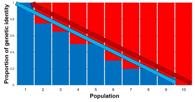
The genetic representation of the above isolation-by-distance example. Each column represents a single population (in the previous figure, a pie chart), with the different colours also representing the relative genetic identity of that population. As you can see, moving from Population 1 to 10 leads to a gradient (decreasing) in blue genes but increase in red genes. The inverse can be said moving in the opposite direction. That said, comparing Population 1 and Population 10 shows that they’re clearly different, although there is no clear cut-off point across the range of other populations.

Medium dispersal capabilities are also often a requirement for forming ‘metapopulations’. In this population arrangement, several semi-independent populations are present within the geographic range of the species. Each of these are subject to their own local environmental pressures and demographic dynamics, and because of this may go locally extinct at any given time. However, dispersal connections between many of these populations leads to recolonization and gene flow patterns, allowing for extinction-dispersal dynamics to sustain the overall metapopulation. Generally, this would require greater levels of dispersal than those typically found within metapopulation species, as individuals must traverse uninhabitable regions relatively frequently to recolonise locally extinct habitat.

Metapopulation structure.jpg
An example of metapopulation dynamics. Different subpopulations (lettered circles) are connected via dispersal (arrows). These different subpopulations can be different sizes and are mostly independent of one another, meaning that a single subpopulation can go locally extinct (the red X) without collapsing the entire system. The different dispersal pathways mean that one population can recolonise extinct habitat and essentially ‘rebirth’ other subpopulations (the green arrows).

Weakly dispersing species

At the far opposite end of the dispersal ability spectrum, we have low dispersal species. These are often localised, endemic species that for various reasons might be unable to travel very far at all; for some, they may spend their entire adult life in a sedentary form. The lack of dispersal lends to very strong levels of population structure, and individual populations often accumulate genetic differences relatively quickly due to genetic drift or local adaptation.

Species with low dispersal capabilities are often at risk of local extinction and are unable to easily recolonise these habitats after the event has ended. Their movement is often restricted to rare environmental events such as flooding that carry individuals long distances despite their physiological limitations. Because of this, low dispersal species are often at greater risk of total extinction and extinction vertices than their higher dispersing counterparts.

Accounting for dispersal in population genetics

Incorporating biological and physiological aspects of our study taxa is important for interpreting the evolutionary context of species. Dispersal ability is but one of many characteristics that can influence the ability of species to respond to selective pressures, and the context in which this natural selection occurs. Thus, understanding all aspects of an organism is important in building the full picture of their evolution and future prospects.

Fantastic Genes and Where to Find Them

The genetics of adaptation

Adaptation and evolution by natural selection remains one of the most significant research questions in many disciplines of biology, and this is undoubtedly true for molecular ecology. While traditional evolutionary studies have been based on the physiological aspects of organisms and how this relates to their evolution, such as how these traits improve their fitness, the genetic component of adaptation is still somewhat elusive for many species and traits.

Hunting for adaptive genes in the genome

We’ve previously looked at the two main categories of genetic variation: neutral and adaptive. Although we’ve focused predominantly on the neutral components of the genome, and the types of questions about demographic history, geographic influences and the effect of genetic drift, they cannot tell us (directly) about the process of adaptation and natural selective changes in species. To look at this area, we’d have to focus on adaptive variation instead; that is, genes (or other related genetic markers) which directly influence the ability of a species to adapt and evolve. These are directly under natural selection, either positively (‘selected for’) or negatively (‘selected against’).

Given how complex organisms, the environment and genomes can be, it can be difficult to determine exactly what is a real (i.e. strong) selective pressure, how this is influenced by the physical characteristics of the organism (the ‘phenotype’) and which genes are fundamental to the process (the ‘genotype’). Even determining the relevant genes can be difficult; how do we find the needle-like adaptive genes in a genomic haystack?

Magnifying glass figure
If only it were this easy.

There’s a variety of different methods we can use to find adaptive genetic variation, each with particular drawbacks and strengths. Many of these are based on tests of the frequency of alleles, rather than on the exact genetic changes themselves; adaptation works more often by favouring one variant over another rather than completely removing the less-adaptive variant (this would be called ‘fixation’). So measuring the frequency of different alleles is a central component of many analyses.

FST outlier tests

One of the most classical examples is called an ‘FST outlier test’. This can be a bit complicated without understanding what FST is actually measures: in short terms, it’s a statistical measure of ‘population differentiation due to genetic structure’. The FST value of one particular population can determine how genetically similar it is to another. An FST value of 1 implies that the two populations are as genetically different as they could possibly be, whilst an FST value of 0 implies that they are genetically identical populations.

Generally, FST reflects neutral genetic structure: it gives a background of how, on average, different are two populations. However, if we know what the average amount of genetic differentiation should be for a neutral DNA marker, then we would predict that adaptive markers are significantly different. This is because a gene under selection should be more directly pushed towards or away from one variant (allele) than another, and much more strongly than the neutral variation would predict. Thus, the alleles that are way more or less frequent than the average pattern we might assume are under selection. This is the basis of the FST outlier test; by comparing two or more populations (using FST), and looking at the distribution of allele frequencies, we can pick out a few alleles that vary from the average pattern and suggest that they are under selection (i.e. are adaptive).

There are a few significant drawbacks for FST outlier tests. One of the most major ones is that genetic drift can also produce a large number of outliers; in a small population, for example, one allele might be fixed (has a frequency of 1, with no alternative allele in the population) simply because there is not enough diversity or population size to sustain more alleles. Even if this particular allele was extremely detrimental, it’d still appear to be favoured by natural selection just because of drift.

Drift leading to outliers diagram
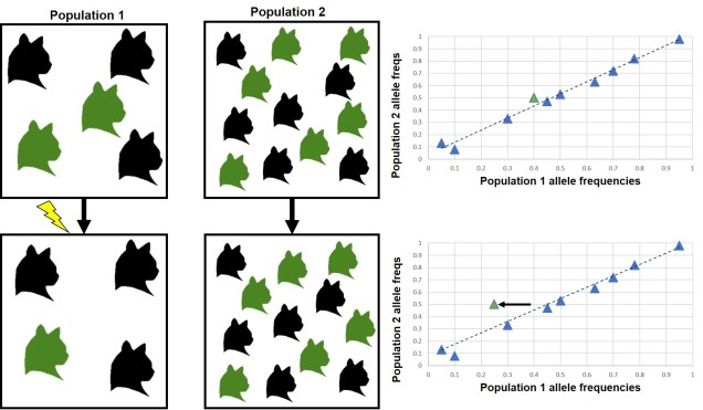
An example of genetic drift leading to outliers, featuring our friends the cat population. Top row: Two cat populations, one small (left; n = 5) and one large (middle, n = 12) show little genetic differentiation between them (right; each triangle represents a single gene or locus; the ‘colour’ gene is marked in green). The average (‘neutral’) pattern of differentiation is shown by the dashed line. Much like in our original example, one cat in the small population is horrifically struck by lightning and dies (RIP again). Now when we compare the frequency of the alleles of the two populations (bottom), we see that (because a green cat died), the ‘colour’ locus has shifted away from the general trend (right) and is now an outlier. Thus, genetic drift in the ‘colour’ gene gives the illusion of a selective loci (even though natural selection didn’t cause the change, since colour does not relate to how likely a cat is to be struck by lightning).

Secondly, the cut-off for a ‘significant’ vs. ‘relatively different but possibly not under selection’ can be a bit arbitrary; some genes that are under weak selection can go undetected. Furthermore, recent studies have shown a growing appreciation for polygenic adaptation, where tiny changes in allele frequencies of many different genes combine together to cause strong evolutionary changes. For example, despite the clear heritable nature of height (tall people often have tall children), there is no clear ‘height’ gene: instead, it appears that hundreds of genes are potentially very minor height contributors.

Polygenic height figure final
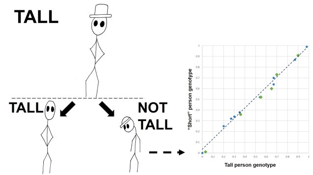
In this example, we have one tall parent (top) who produces two offspring; one who is tall (left) and one who isn’t (right). In order to understand what genetic factors are contributing to their height differences, we compare their genetics (right; each dot represents a single locus). Although there aren’t any particular loci that look massively different between the two, the cumulative effect of tiny differences (the green triangles) together make one person taller than the other. There are no clear outliers, but many (poly) different genes (genic) acting together.

Genotype-environment associations

To overcome these biases, sometimes we might take a more methodological approach called ‘genotype-environment association’. This analysis differs in that we select what we think our selective pressures are: often environmental characteristics such as rainfall, temperature, habitat type or altitude. We then take two types of measures per individual organism: the genotype, through DNA sequencing, and the relevant environmental values for that organisms’ location. We repeat this over the full distribution of the species, taking a good number of samples per population and making sure we capture the full variation in the environment. Then we perform a correlation-type analysis, which seeks to see if there’s a connection or trend between any particular alleles and any environmental variables. The most relevant variables are often pulled out of the environmental dataset and focused on to reduce noise in the data.

The main benefit of GEA over FST outlier tests is that it’s unlikely to be as strongly influenced by genetic drift. Unless (coincidentally) populations are drifting at the same genes in the same pattern as the environment, the analysis is unlikely to falsely pick it up. However, it can still be confounded by neutral population structure; if one population randomly has a lot of unique alleles or variation, and also occurs in a somewhat unique environment, it can bias the correlation. Furthermore, GEA is limited by the accuracy and relevance of the environmental variables chosen; if we pick only a few, or miss the most important ones for the species, we won’t be able to detect a large number of very relevant (and likely very selective) genes. This is a universal problem in model-based approaches and not just limited to GEA analysis.

New spells to find adaptive genes?

It seems likely that with increasing datasets and better analytical platforms, many more types of analysis will be developed to delve deeper into the adaptive aspects of the genome. With whole-genome sequencing starting to become a reality for non-model species, better annotation of current genomes and a steadily increasing database of functional genes, the ability of researchers to investigate evolution and adaptation at the genomic level is also increasing.