Unravelling the evolutionary history of organisms – one of the main goals of phylogenetic research – remains a challenging prospect due to a number of theoretical and analytical aspects. Particularly, trying to reconstruct evolutionary patterns based on current genetic data (the most common way phylogenetic trees are estimated) is prone to the erroneous influence of some secondary factors. One of these is referred to as ‘incomplete lineage sorting’, which can have a major effect on how phylogenetic relationships are estimated and the statistical confidence we may have around these patterns. Today, we’re going to take a look at incomplete lineage sorting (shortened to ILS for brevity herein) using a game-based analogy – a Pachinko machine. Or, if you’d rather, the same general analogy also works for those creepy clown carnival games, but I prefer the less frightening alternative.
A recurring analytical method, both within The G-CAT and the broader ecological genetic literature, is based on coalescent theory. This is based on the mathematical notion that mutations within genes (leading to new alleles) can be traced backwards in time, to the point where the mutation initially occurred. Given that this is a retrospective, instead of describing these mutation moments as ‘divergence’ events (as would be typical for phylogenetics), these appear as moments where mutations come back together i.e. coalesce.
Before we can explore the multitude of applications of the coalescent, we need to understand the fundamental underlying model. The initial coalescent model was described in the 1980s, built upon by a number of different ecologists, geneticists and mathematicians. However, John Kingman is often attributed with the formation of the original coalescent model, and the Kingman’s coalescent is considered the most basic, primal form of the coalescent model.
From a mathematical perspective, the coalescent model is actually (relatively) simple. If we sampled a single gene from two different individuals (for simplicity’s sake, we’ll say they are haploid and only have one copy per gene), we can statistically measure the probability of these alleles merging back in time (coalescing) at any given generation. This is the same probability that the two samples share an ancestor (think of a much, much shorter version of sharing an evolutionary ancestor with a chimpanzee).
Normally, if we were trying to pick the parents of our two samples, the number of potential parents would be the size of the ancestral population (since any individual in the previous generation has equal probability of being their parent). But from a genetic perspective, this is based on the genetic (effective) population size (Ne), multiplied by 2 as each individual carries two copies per gene (one paternal and one maternal). Therefore, the number of potential parents is 2Ne.
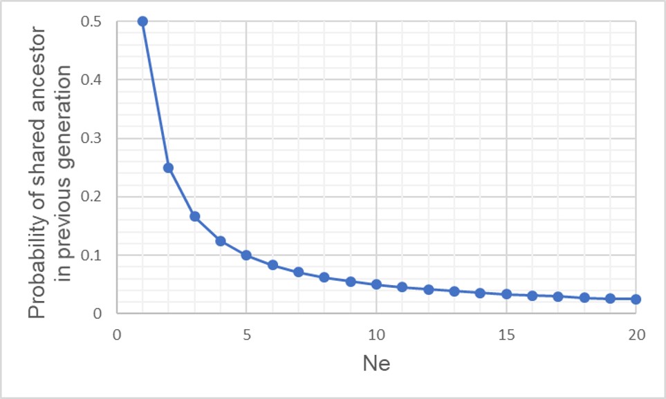
A graph of the probability of a coalescent event (i.e. two alleles sharing an ancestor) in the immediatelypreceding generation (i.e. parents) relatively to the size of the population. As one might expect, with larger population sizes there is low chance of sharing an ancestor in the immediately prior generation, as the pool of ‘potential parents’ increases.
If we have an idealistic population, with large Ne, random mating and no natural selection on our alleles, the probability that their ancestor is in this immediate generation prior (i.e. share a parent) is 1/(2Ne). Inversely, the probability they don’t share a parent is 1 − 1/(2Ne). If we add a temporal component (i.e. number of generations), we can expand this to include the probability of how many generations it would take for our alleles to coalesce as (1 – (1/2Ne))t-1 x 1/2Ne.
The probability of two alleles sharing a coalescent event back in time under different population sizes. Similar to above, there is a higher probability of an earlier coalescent event in smaller populations as the reduced number of ancestors means that alleles are more likely to ‘share’ an ancestor. However, over time this pattern consistently decreases under all population size scenarios.
Although this might seem mathematically complicated, the coalescent model provides us with a scenario of how we would expect different mutations to coalesce back in time if those idealistic scenarios are true. However, biology is rarely convenient and it’s unlikely that our study populations follow these patterns perfectly. By studying how our empirical data varies from the expectations, however, allows us to infer some interesting things about the history of populations and species.
A diagram of how the coalescent can be used to detect bottlenecks in a single population (centre). In this example, we have contemporary population in which we are tracing the coalescence of two main alleles (red and green, respectively). Each circle represents a single individual (we are assuming only one allele per individual for simplicity, but for most animals there are up to two). Looking forward in time, you’ll notice that some red alleles go extinct just before the bottleneck: they are lost during the reduction in Ne. Because of this, if we measure the rate of coalescence (right), it is much higher during the bottleneck than before or after it. Another way this could be visualised is to generate gene trees for the alleles (left): populations that underwent a bottleneck will typically have many shorter branches and a long root, as many branches will be ‘lost’ by extinction (the dashed lines, which are not normally seen in a tree).
This makes sense from theoretical perspective as well, since strong genetic bottlenecks means that most alleles are lost. Thus, the alleles that we do have are much more likely to coalesce shortly after the bottleneck, with very few alleles that coalesce before the bottleneck event. These alleles are ones that have managed to survive the purge of the bottleneck, and are often few compared to the overarching patterns across the genome.
Testing migration (gene flow) across lineages
Another demographic factor we may wish to test is whether gene flow has occurred across our populations historically. Although there are plenty of allele frequency methods that can estimate contemporary gene flow (i.e. within a few generations), coalescent analyses can detect patterns of gene flow reaching further back in time.
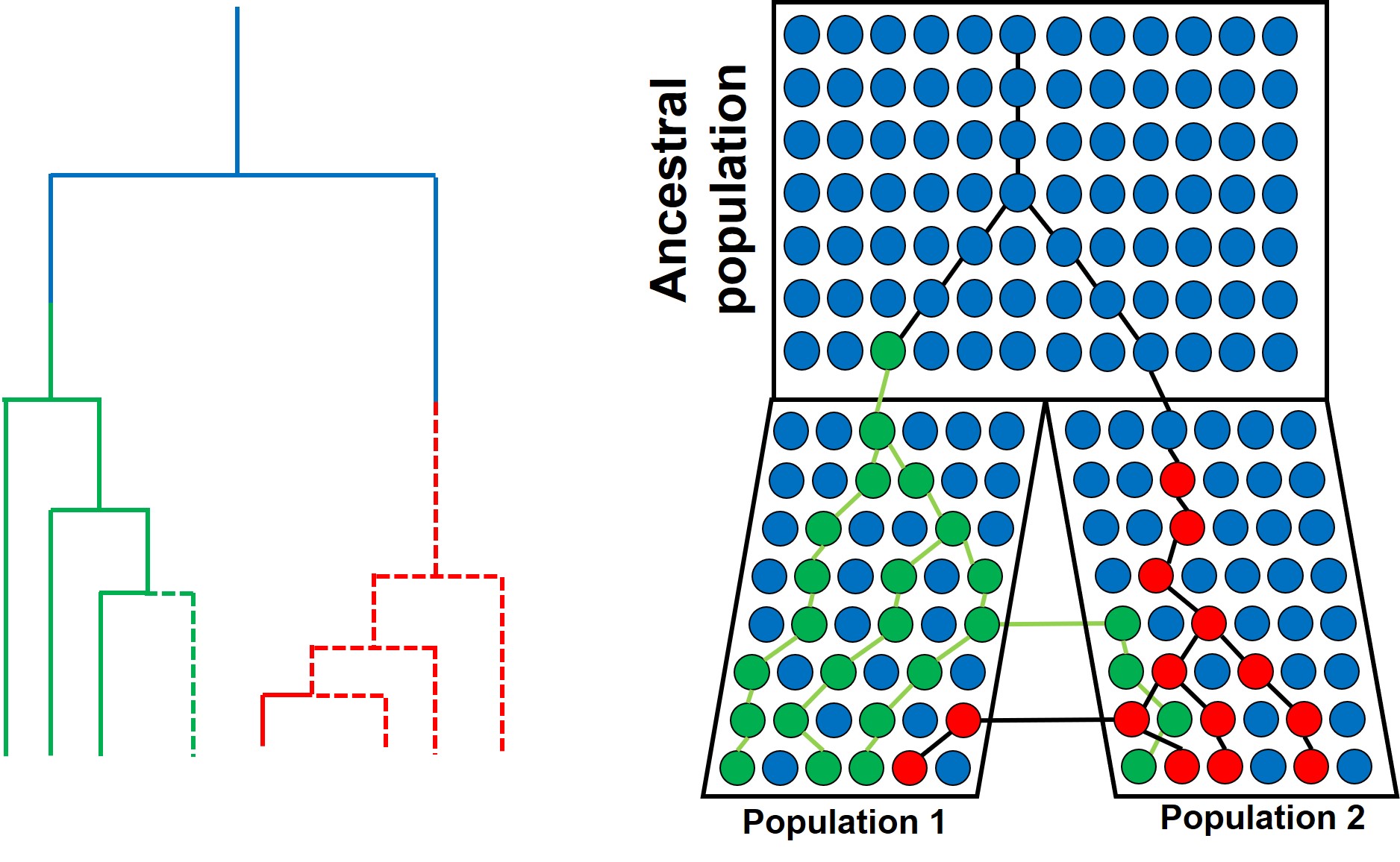
A similar model of coalescence as above, but testing for migration rate (gene flow) in two recently diverged populations (right). In this example, when we trace two alleles (red and green) back in time, we notice that some individuals in Population 1 coalesce more recently with individuals of Population 2 than other individuals of Population 1 (e.g. for the red allele), and vice versa for the green allele. This can also be represented with gene trees (left), with dashed lines representing individuals from Population 2 and whole lines representing individuals from Population 1. This incomplete split between the two populations is the result of migration transferring genes from one population to the other after their initial divergence (also called ‘introgression’ or ‘horizontal gene transfer’).
Testing divergence time
In a similar vein, the coalescent can also be used to test how long ago the two contemporary populations diverged. Similar to gene flow, this is often included as an additional parameter on top of the coalescent model in terms of the number of generations ago. To convert this to a meaningful time estimate (e.g. in terms of thousands or millions of years ago), we need to include a mutation rate (the number of mutations per base pair of sequence per generation) and a generation time for the study species (how many years apart different generations are: for humans, we would typically say ~20-30 years).
An example of using the coalescent to test the divergence time between two populations, this time using three different alleles (red, green and yellow). Tracing back the coalescence of each alleles reveals different times (in terms of which generation the coalescence occurs in) depending on the allele (right). As above, we can look at this through gene trees (left), showing variation how far back the two populations (again indicated with bold and dashed lines respectively) split. The blue box indicates the range of times (i.e. a confidence interval) around which divergence occurred: with many more alleles, this can be more refined by using an ‘average’ and later related to time in years with a generation time.
While each of these individual concepts may seem (depending on how well you handle maths!) relatively simple, one critical issue is the interactive nature of the different factors. Gene flow, divergence time and population size changes will all simultaneously impact the distribution and frequency of alleles and thus the coalescent method. Because of this, we often use complex programs to employ the coalescent which tests and balances the relative contributions of each of these factors to some extent. Although the coalescent is a complex beast, improvements in the methodology and the programs that use it will continue to improve our ability to infer evolutionary history with coalescent theory.
A number of timesbefore on The G-CAT, we’ve discussed the idea of using the frequency of different genetic variants (alleles) within a particular population or species to test a number of different questions about evolution, ecology and conservation. These are all based on the central notion that certain forces of nature will alter the distribution and frequency of alleles within and across populations, and that these patterns are somewhat predictable in how they change.
One particular distinction we need to make early here is the difference between allele frequency and allele identity. In these analyses, often we are working with the same alleles (i.e. particular variants) across our populations, it’s just that each of these populations may possess these particular alleles in different frequencies. For example, one population may have an allele (let’s call it Allele A) very rarely – maybe only 10% of individuals in that population possess it – but in another population it’s very common and perhaps 80% of individuals have it. This is a different level of differentiation than comparing how different alleles mutate (as in the coalescent) or how these mutations accumulate over time (like in many phylogenetic-based analyses).
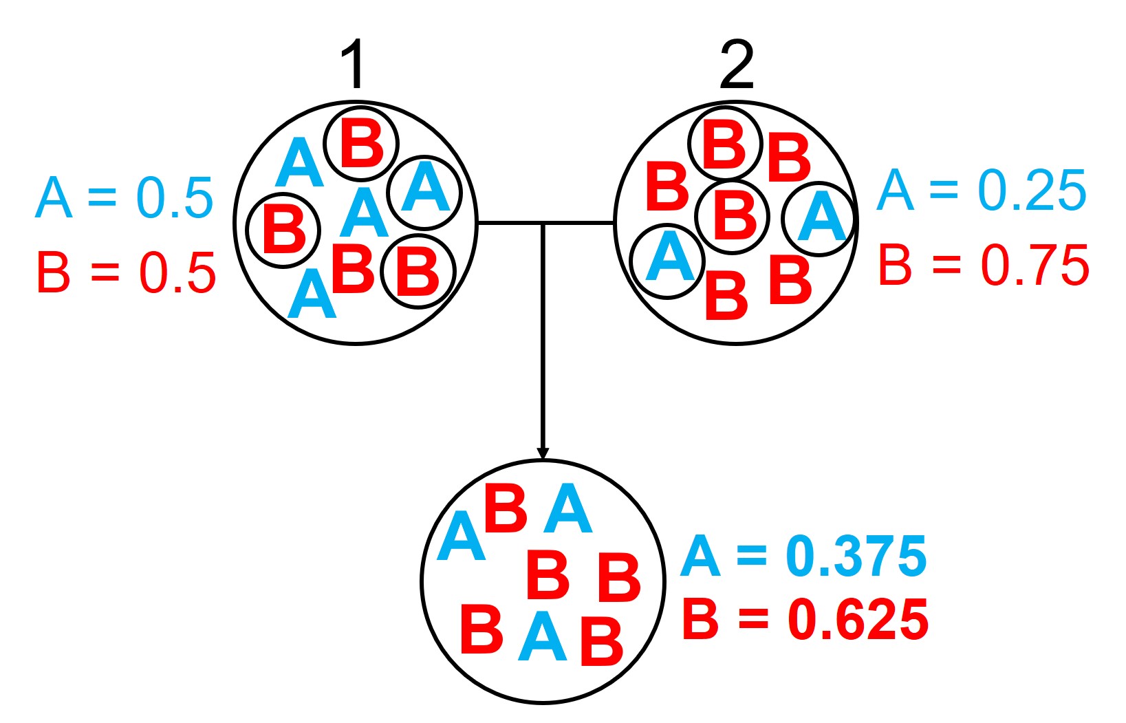
An example of the difference between allele frequency and identity.In this example (and many of the figures that follow in this post), the circle denote different populations, within which there are individuals which possess either an A gene (blue) or a B gene. Left: If we compared Populations 1 and 2, we can see that they both have A and B alleles. However, these alleles vary in their frequency within each population, with an equal balance of A and B in Pop 1 and a much higher frequency of B in Pop 2. Right: However, when we compared Pop 3 and 4, we can see that not only do they vary in frequencies, they vary in the presence of alleles, with one allele in each population but not the other.
An example of how gene flow across populations homogenises allele frequencies. We start with two initial populations (1 and 2 from above), which have very different allele frequencies. Hybridising individuals across the two populations means some alleles move from Pop 1 and Pop 2 into the hybrid population: which alleles moves is random (the smaller circles). Because of this, the resultant hybrid population has an allele frequency somewhere in between the two source populations: think of like mixing red and blue cordial and getting a purple drink.
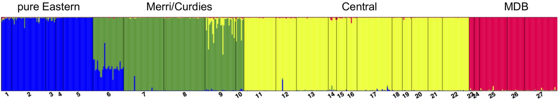
An example of a Structure plot which long-term The G-CAT readers may be familiar with. This is taken from Brauer et al. (2013), where the authors studied the population structure of the Yarra pygmy perch. Each small column represents a single individual, with the colours representing how well the alleles of that individual fit a particular genetic population (each population has one colour). The numbers and broader columns refer to different ‘localities’ (different from populations) where individuals were sourced. This shows clear strong population structure across the 4 main groups, except for in Locality 6 where there is a mixture of Eastern and Merri/Curdies alleles.
Determining genetic bottlenecks and demographic change
A diagram of how allele frequencies change in genetic bottlenecks due to genetic drift. Left: Large circles again denote a population (although across different sequential times), with smaller circle denoting which alleles survive into the next generation (indicated by the coloured arrows). We start with an initial ‘large’ population of 8, which is reduced down to 4 and 2 in respective future times. Each time the population contracts, only a select number of alleles (or individuals) ‘survive’: assuming no natural selection is in process, this is totally random from the available gene pool. Right: We can see that over time, the frequencies of alleles A and B shift dramatically, leading to the ‘extinction’ of Allele B due to genetic drift. This is because it is the less frequent allele of the two, and in the smaller population size has much less chance of randomly ‘surviving’ the purge of the genetic bottleneck.
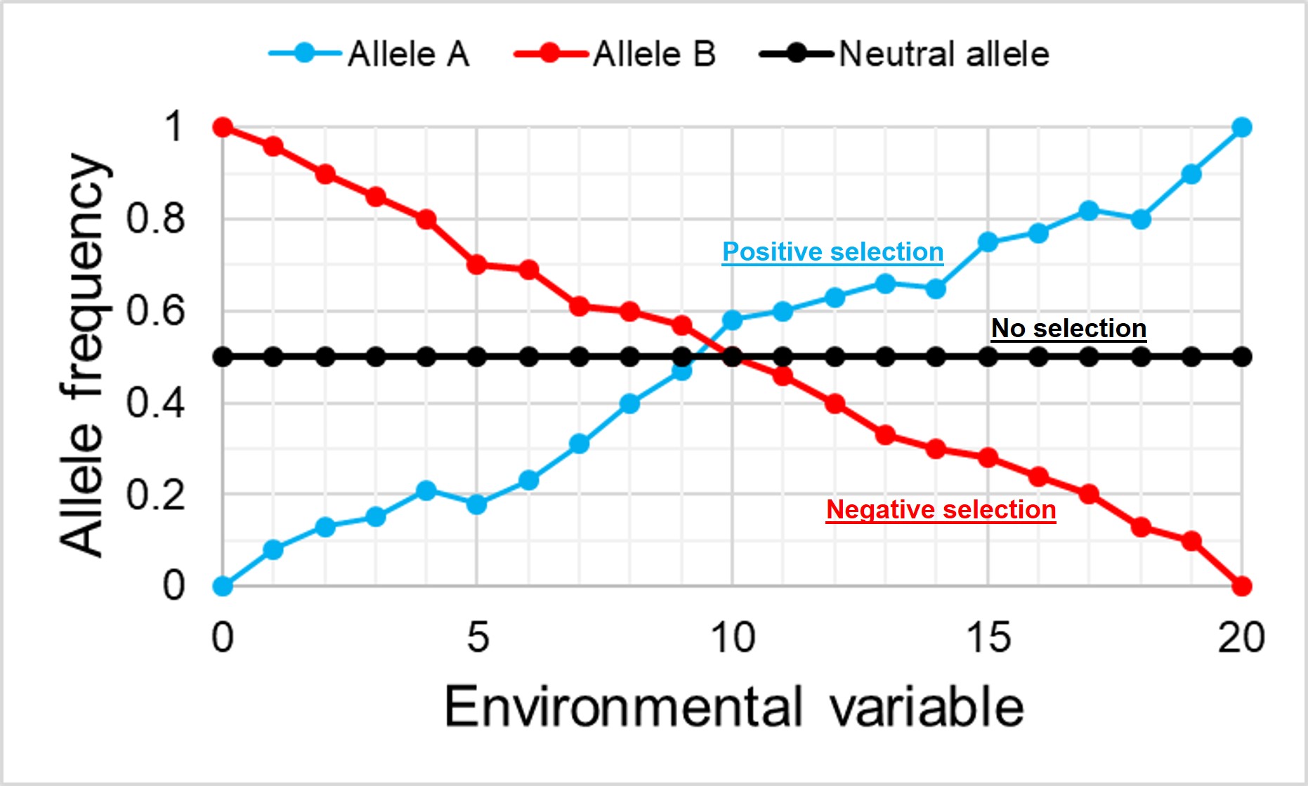
An example of how the frequency of alleles might vary under natural selection in correlation to the environment. In this example, the blue allele A is adaptive and under positive selection in the more intense environment, and thus increases in frequency at higher values. Contrastingly, the red allele B is maladaptive in these environments and decreases in frequency. For comparison, the black allele shows how the frequency of a neutral (non-adaptive or maladaptive) allele doesn’t vary with the environment, as it plays no role in natural selection.
Fixed differences are sometimes used as a type of diagnostic trait for species. This means that each ‘species’ has genetic variants that are not shared at all with its closest relative species, and that these variants are so strongly under selection that there is no diversity at those loci. Often, fixed differences are considered a level above populations that differ by allelic frequency only as these alleles are considered ‘diagnostic’ for each species.
An example of the difference between fixed differences and allelic frequency differences. In this example, we have 5 cats from 3 different species, sequencing a particular target gene. Within this gene, there are three possible alleles: T, A or G respectively. You’ll quickly notice that the T allele is both unique to Species A and is present in all cats of that species (i.e. is fixed). This is a fixed difference between Species A and the other two. Alleles A and G, however, are present in both Species B and C, and thus are not fixed differences even if they have different frequencies.
To distinguish between the two, we often use the overall frequency of alleles in a population as a basis for determining how likely two individuals share an allele by random chance. If alleles which are relatively rare in the overall population are shared by two individuals, we expect that this similarity is due to family structure rather than population history. By factoring this into our relatedness estimates we can get a more accurate overview of how likely two individuals are to be related using genetic information.
The wild world of allele frequency
Despite appearances, this is just a brief foray into the many applications of allele frequency data in evolution, ecology and conservation studies. There are a plethora of different programs and methods that can utilise this information to address a variety of scientific questions and refine our investigations.
Although we often focus on the genetic traits of species in molecular ecology studies, the physiological (or phenotypic) traits are equally as important in shaping their evolution. These different traits are not only the result themselves of evolutionary forces but may further drive and shape evolution into the future by changing how an organism interacts with the environment.
There are a massive number of potential traits we could focus on, each of which could have a large number of different (and interacting) impacts on evolution. One that is often considered, and highly relevant for genetic studies, is the influence of dispersal capability.
Dispersal
Dispersal is essentially the process of an organism migrating to a new habitat, to the point of the two being used almost interchangeably. Often, however, we regard dispersal as a migration event that actually has genetic consequences; particularly, if new populations are formed or if organisms move from one population to another. This can differ from straight migration in that animals that migrate might not necessarily breed (and thus pass on genes) into a new region during their migration; thus, evidence of those organisms will not genetically proliferate into the future through offspring.
Naturally, the ability of organisms to disperse is highly variable across the tree of life and reliant on a number of other physiological factors. Marine mammals, for example, can disperse extremely far throughout their lifetimes, whereas some very localised species like some insects may not move very far within their lifetime at all. The movement of organisms directly facilitates the movement of genetic material, and thus has significant impacts on the evolution and genetic diversity of species and populations.
The (simplistic) relationship between dispersal capability and one aspect of population genetics, population structure (measured as Fst). As organisms are more capable of dispersing longer distance (or more frequently), the barriers between populations become weaker.
As these individuals occupy large ranges, localised impacts are unlikely to critically affect their full distribution. Individual organisms that are occupying an unpleasant space can easily move to a more favourable habitat (provided that one exists). Furthermore, with a large population (which is more likely with highly dispersive species), genetic drift is substantially weaker and natural selection (generally) has a higher amount of genetic diversity to work with. This is, of course, assuming that dispersal leads to a large overall population, which might not be the case for species that are critically endangered (such as the cheetah).
The Wright island model of population structure. In this example, different independent populations are labelled in the bold letters, with dispersal pathways demonstrated by the different arrows. In the island model, dispersal is equally likely between all populations (including from B–D in this example, even though there aren’t any arrows showing it). Naturally, this is not overly realistic and so the island model is used mostly as a neutral, base model.
Intermediately dispersing species
A large number of species, however, are likely to occupy a more intermediate range of dispersal ability. These species might be able to migrate to neighbouring populations, or across a large proportion of their geographic range, but individuals from one end of the range are still somewhat isolated from individuals at the other end.
This often leads to some effect of population structure; different portions of the geographic range are genetically segregated from one another depending on how much gene flow (i.e. dispersal) occurs between populations. In the most simplest scenario, this can lead to what we call isolation-by-distance. Rather than forming totally independent populations, gene flow occurs across short ranges between adjacent ‘populations’. This causes a gradient of genetic differentiation, with one end of the range being clearly genetically different to the other end, with a gradual slope throughout the range. We see this often in marine invertebrates, for example, which might have somewhat localised dispersal but still occupy a large range by following oceanographic currents.
An example of how an isolation-by-distance population network might come about. In this example, we have a series of populations (the different pie charts) spread throughout a river system (that blue thing). The different pie charts represent how much of the genetics of that population matches one end of the river: either the blue end (left) or red end (right). Populations can easily disperse into adjacent populations (the green arrows) but less so to further populations. This leads to gradual changes across the length of the river, with the far ends of the river clearly genetically distinct from the opposite end but relatively similar to neighbouring populations.
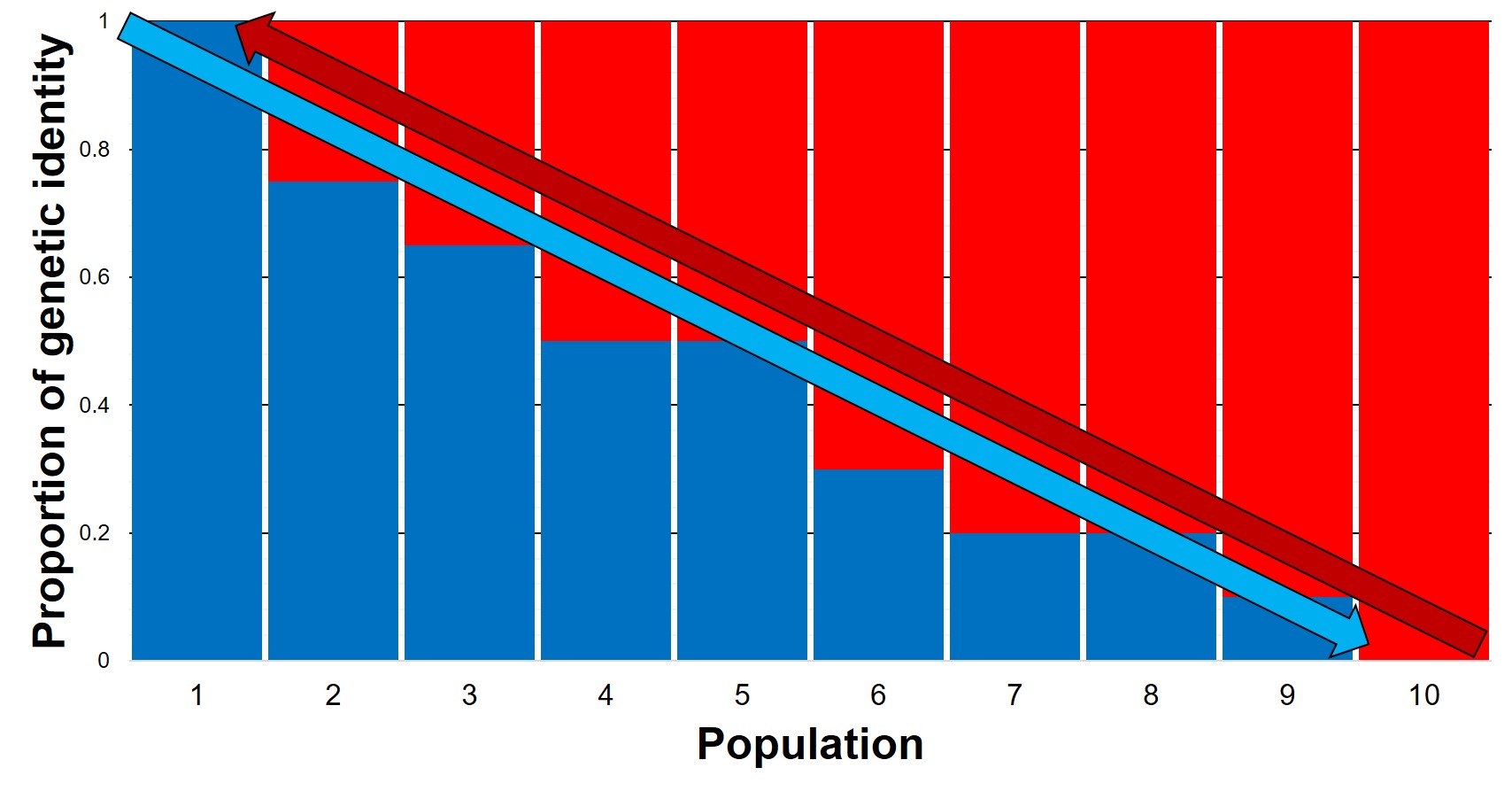
The genetic representation of the above isolation-by-distance example. Each column represents a single population (in the previous figure, a pie chart), with the different colours also representing the relative genetic identity of that population. As you can see, moving from Population 1 to 10 leads to a gradient (decreasing) in blue genes but increase in red genes. The inverse can be said moving in the opposite direction. That said, comparing Population 1 and Population 10 shows that they’re clearly different, although there is no clear cut-off point across the range of other populations.
Medium dispersal capabilities are also often a requirement for forming ‘metapopulations’. In this population arrangement, several semi-independent populations are present within the geographic range of the species. Each of these are subject to their own local environmental pressures and demographic dynamics, and because of this may go locally extinct at any given time. However, dispersal connections between many of these populations leads to recolonization and gene flow patterns, allowing for extinction-dispersal dynamics to sustain the overall metapopulation. Generally, this would require greater levels of dispersal than those typically found within metapopulation species, as individuals must traverse uninhabitable regions relatively frequently to recolonise locally extinct habitat.
An example of metapopulation dynamics. Different subpopulations (lettered circles) are connected via dispersal (arrows). These different subpopulations can be different sizes and are mostly independent of one another, meaning that a single subpopulation can go locally extinct (the red X) without collapsing the entire system. The different dispersal pathways mean that one population can recolonise extinct habitat and essentially ‘rebirth’ other subpopulations (the green arrows).
Species with low dispersal capabilities are often at risk of local extinction and are unable to easily recolonise these habitats after the event has ended. Their movement is often restricted to rare environmental events such as flooding that carry individuals long distances despite their physiological limitations. Because of this, low dispersal species are often at greater risk of total extinction and extinction vertices than their higher dispersing counterparts.
Accounting for dispersal in population genetics
Incorporating biological and physiological aspects of our study taxa is important for interpreting the evolutionary context of species. Dispersal ability is but one of many characteristics that can influence the ability of species to respond to selective pressures, and the context in which this natural selection occurs. Thus, understanding all aspects of an organism is important in building the full picture of their evolution and future prospects.