Mutation

The neutral theory

Many, many times within The G-CAT we’ve discussed the difference between neutral and selective processes, DNA markers and their applications in our studies of evolution, conservation and ecology. The idea that many parts of the genome evolve under a seemingly random pattern – largely dictated by genome-wide genetic drift rather than the specific force of natural selection – underpins many demographic and adaptive (in outlier tests) analyses.

This is based on the idea that for genes that are not related to traits under selection (either positively or negatively), new mutations should be acquired and lost under predominantly random patterns. Although this accumulation of mutations is influenced to some degree by alternate factors such as population size, the overall average of a genome should give a picture that largely discounts natural selection. But is this true? Is the genome truly neutral if averaged?

Non-neutrality

First, let’s take a look at what we mean by neutral or not. For genes that are not under selection, alleles should be maintained at approximately balanced frequencies and all non-adaptive genes across the genome should have relatively similar distribution of frequencies. While natural selection is one obvious way allele frequencies can be altered (either favourably or detrimentally), other factors can play a role.

As stated above, population sizes have a strong impact on allele frequencies. This is because smaller populations are more at risk of losing rarer alleles due to random deaths (see previous posts for a more thorough discussion of this). Additionally, genes which are physically close to other genes which are under selection may themselves appear to be under selection due to linkage disequilibrium (often shortened to ‘LD’). This is because physically close genes are more likely to be inherited together, thus selective genes can ‘pull’ neighbours with them to alter their allele frequencies.

Linkage disequilibrium figure — An example of how linkage disequilibrium can alter allele frequency of ‘neutral’ parts of the genome as well. In this example, only one part of this section of the genome is selected for: the **green gene**. Because of this positive selection, the frequency of a particular allele at this gene increases (the **blue graph**): however, nearby parts of the genome also increase in frequency due to their proximity to this selected gene, which decreases with distance. The extent of this effect determines the size of the ‘linkage block’ (see below).

Why might ‘neutral’ models not be neutral?

The assumption that the vast majority of the genome evolves under neutral patterns has long underpinned many concepts of population and evolutionary genetics. But it’s never been all that clear exactly how much of the genome is actually evolving neutrally or adaptively. How far natural selection reaches beyond a single gene under selection depends on a few different factors: let’s take a look at a few of them.

Linked selection

As described above, physically close genes (i.e. located near one another on a chromosome) often share some impacts of selection due to reduced recombination that occurs at that part of the genome. In this case, even alleles that are not adaptive (or maladaptive) may have altered frequencies simply due to their proximity to a gene that is under selection (either positive or negative).

Recombination blocks and linkage figure — A (perhaps familiar) example of the interaction between recombination (the breaking and mixing of different genes across chromosomes) and linkage disequilibrium. In this example, we have 5 different copies of a part of the genome (**different coloured sequences**), which we randomly ‘break’ into separate fragments (**breaks indicated by the dashed lines**). If we focus on a particular base in the sequence (the **yellow A**) and count the number of times a particular base pair is on the same fragment, we can see how physically close bases are more likely to be coinherited than further ones (**bottom column graph**). This makes mathematical sense: if two bases are further apart, you’re more likely to have a break that separates them. This is the very basic underpinning of linkage and recombination, and the size of the region where bases are likely to be coinherited is called the ‘linkage block’.

Under these circumstances, for a region of a certain distance (dubbed the ‘linkage block’) around a gene under selection, the genome will not truly evolve neutrally. Although this is simplest to visualise as physically linked sections of the genome (i.e. adjacent), linked genes do not necessarily have to be next to one another, just linked somehow. For example, they may be different parts of a single protein pathway.

The extent of this linkage effect depends on a number of other factors such as ploidy (the number of copies of a chromosome a species has), the size of the population and the strength of selection around the central locus. The presence of linkage and its impact on the distribution of genetic diversity (LD) has been well documented within evolutionary and ecological genetic literature. The more pressing question is one of extent: how much of the genome has been impacted by linkage? Is any of the genome unaffected by the process?

Background selection

One example of linked selection commonly used to explain the proliferation of non-neutral evolution within the genome is ‘background selection’. Put simply, background selection is the purging of alleles due to negative selection on a linked gene. Sometimes, background selection is expanded to include any forms of linked selection.

Under the first etymology of background selection, the process can be divided into two categories based on the impact of the linkage. As above, one scenario is the purging of neutral alleles (and therefore reduction in genetic diversity) as it is associated with a deleterious maladaptive gene nearby. Contrastingly, some neutral alleles may be preserved by association with a positively selected adaptive gene: this is often referred to as ‘genetic hitchhiking’ (which I’ve always thought was kind of an amusing phrase…).

Genetic hitchhiking picture.jpg — Definitely not how genetic hitchhiking works.

The presence of background selection – particularly under the ‘maladaptive’ scenario – is often used as a counter-argument to the ‘paradox in variation’. This paradox was determined by evolutionary biologist Richard Lewontin, who noted that despite massive differences in population sizes across the many different species on Earth, the total amount of ‘neutral’ genetic variation does not change significantly. In fact, he observed no clear relationship (directly) between population size and neutral variation. Many years after this observation, the influence of background selection and genetic hitchhiking on the distribution of genomic diversity helps to explain how the amount of neutral genomic variation is ‘managed’, and why it doesn’t vary excessively across biota.

What does it mean if neutrality is dead?

This findings have significant implications for our understanding of the process of evolution, and how we can detect adaptation within the genome. In light of this research, there has been heated discussion about whether or not neutral theory is ‘dead’, or a useful concept.

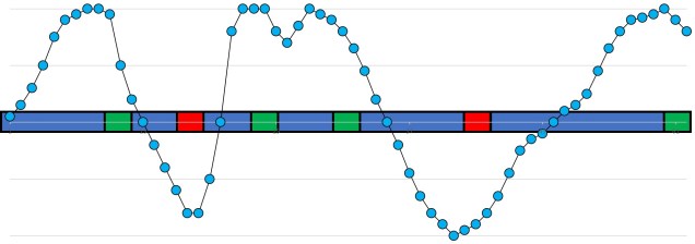
Genome wide allele frequency figure.jpg — A vague summary of how a large portion of the genome might not actually be neutral. In this section of the genome, we have neutral (**blue**), maladaptive (**red**) and adaptive (**green**) elements. Natural selection either favours, disfavours, or is ambivalent about each of this sections alone. However, there is significant ‘spill-over’ around regions of positively or negatively selected sections, which causes the allele frequency of even the neutral sections to fluctuate widely. The **blue dotted line** represents this: when the line is above the genome, allele frequency is increased; when it is below it is decreased. As we travel along this section of the genome, you may notice it is rarely ever in the middle (the so-called ‘neutral‘ allele frequency, in line with the genome).

Although I avoid having a strong stance here (if you’re an evolutionary geneticist yourself, I will allow you to draw your own conclusions), it is my belief that the model of neutral theory – and the methods that rely upon it – are still fundamental to our understanding of evolution. Although it may present itself as a more conservative way to identify adaptation within the genome, and cannot account for the effect of the above processes, neutral theory undoubtedly presents itself as a direct and well-implemented strategy to understand adaptation and demography.

Adaptation is arguably the most critical biological process in the evolution of species. The process of evolution by natural selection is the cornerstone of evolutionary biology (and indeed, all of contemporary biology!) and adaptation remains fundamental to the process. We know that adaptation is based on the idea that some genetic variants are ‘better’ adapted than others, and thus are unequally shared across a population. But where does this genetic variation come from?

The accumulation of new genetic variation

The classic way for new genetic variants to appear is often thought of as mutation: changes in a single base in the DNA are caused by various external processes such as chemical, physical or environmental influences (such as the sci-fi classics like UV rays or toxic chemicals). Although these forms of mutations happen very rarely and certainly don’t have the same effects comic books would leave you to believe, new mutations can occur relatively rapidly depending on the characteristics of the species. However, the most common way for new mutations to occur is actually part of the DNA replication process: copying DNA is not always perfect and even though the relevant proteins essentially run a spellcheck, sometimes the copy is not 100% perfect and new mutations occur.

Adaptation of mutation figure — An example of how adaptation can occur from a new mutation. In this example, we have one gene (TTXTT), with initial only one allele (variant), TTATT. In the second generation (row), a mutation occurs in one individual which creates a new, second allele: TTGTT. This allele is favoured over the TTATT allele, and in the next generation it’s frequency increases as the alternative allele frequency decreases (the pattern is shown in the frequency values on the right side).

It is important to remember that only mutations that are present in the reproductive cells (sperm and eggs) can be inherited and passed on, and thus be a source for adaptation. Mutations in other tissues of the body, such as within the skin, are not spread across the entire body of the subject and thus aren’t passed on to offspring.

Standing genetic variation

Alternatively, genetic variation might already be present within a species or population. This is more likely if population sizes are large and populations are well connected and interbreeding. We refer to this diverse initial gene pool as ‘standing genetic variation’: that is, the amount of genetic variation within the population or species before the selective pressure requiring adaptation. Standing genetic variation can be thought of as the ‘diversity of choices’ for natural selection to act upon: the variants are readily available, and if a good choice exists it will be favoured by natural selection and become more widespread within the population or species (i.e. evolve).

Adaptation of standing variation figure.jpg — A slightly more complex example of how adaptation can occur from standing variation, this time with two different genes. One codes for fur colour, with two different alleles: GCATA codes for orange fur, and GCGTA codes for grey fur. The other gene codes for ear tufts, with TTCCT coding for tufts and TCCCT coding for no tufts. Natural selection favours both orange fur and tufted ears, and cats with these traits reproduce more frequently than those without (see graph below). These cats probably look familiar.

Graph of standing variation.jpg — The frequency of all four alleles (i.e. either allele for both genes) over the generations in the above figure. Clearly, we can see how adaptation rapidly favours orange fur and tufted ears over grey fur and non-tufted ears with the shifts in frequencies over the different alleles.

We’ve discussed standing genetic variation before on The G-CAT, but often in a different light (and phrasing). For example, when we’ve talked about founder effect: that is, when a population is formed from only a few different individuals which causes it to be very genetically depauperate. In populations under strong founder effect, there is very little standing genetic variation for natural selection to act upon. This has long been an enigma for many pest species: how have they managed to proliferate so widely when they often originate from so few individuals and lack genetic diversity?

Adaptive variation

Adaptation may not require new genetic variants to be generated from mutation. If there are a large number of alleles within the gene pool to start with, then natural selection may favour one of those variants over others and allow adaptation to start immediately. Compared to the rate at which new mutations occur, are potentially corrected for in DNA repair, are potentially erased by genetic drift, and then put under selective pressure, adaptation from standing genetic variation can occur very quickly.

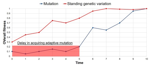
Rate of adaptation figure.jpg — A rough example of the speed of adaptation depending on how the adaptive allele originated: whether it was already present (in the form of standing variation), or whether it was created by a new mutation. As one would expect, there is a significant lag delay in adaptation in the mutation scenario, based on the time it takes for said adaptive mutation to be created through relatively random processes. Thus, a positively selected allele from standing variation can allow a species to adapt much faster than waiting for a positive mutation to occur.

Conserving genetic variation

Given the adaptive potential provided by maintaining a good amount of standing genetic variation, it is imperative to conserve genetic diversity within populations in conservation efforts. This is why we often equate genetic diversity with ‘adaptive potential’ of species, although the exact amount of genetic diversity required for adaptive potential depends on a large number of other factors. Clearly, in some instances species show the ability to adapt to new pressures or novel environments even without a large amount of standing genetic variation.

It is important to remember that standing genetic variation consists of two types: neutral genetic diversity, which is not necessarily under selection at the time, and adaptive genetic diversity, which is directly under selection (although this can be either for or against the given variant). However, currently neutral genetic variants may become adaptive variants in the future if selective pressures change: although those different variants aren’t necessarily beneficial or detrimental at the moment, that may change in the future. Thus, conserving both types of genetic diversity is important for the survivability and longevity of populations under conservation programs.

Other types of adaptation

Although genetic diversity is clearly critically important for adaptive potential, alternative mechanisms for adaptation also exist. One of these relies less on the actual genetic variants being different, but rather how individual genes are used. This can happen in a few different ways, but mostly commonly this is through alternative splicing: when a gene is being ‘read’ and a protein is produced, different parts of the gene can be used (and in different order) to make a completely different protein.

Alternate splicing figure.jpg — An extreme example of alternate splicing of one gene. We start with a single gene, composed of 5 (A–E) main gene elements (exons). Different environmental pressures (like fire risk, flooding, cold weather or predators, for example) cause the organism to use different combinations of these exons to make different proteins (right side; A–D). Actual alternate splicing is not usually this straight-forward (one gene doesn’t conveniently split into four forms depending on the threat), but the process is generally the same.

Believe it or not, we’ve sort of discussed the effects of alternative splicing before. Phenotypic plasticity occurs when a single organism can have very different physiological traits depending on the environment: even though the genes are the same, they are utilised in different ways to make a different body shape. This is how some species can look incredibly different when they live in different places even if they’re genetically very similar. That said, for the vast majority of species maintaining good levels of genetic diversity is critical for the survivability of said species.

The G-cat

Dive head-first into the science of conservation, ecology, evolution and genetics

The reality of neutrality