In more fishy news, this week the latest (and last!) chapter of my PhD, describing how millions of years of climatic stability have allowed isolated and divergent lineages of pygmy perches to persist, was published (Open Access) in Heredity. It covers population divergence, phylogenetic relationships (including estimation of divergence times), species delimitation and projections of species distributions from the past (up to three million years ago) into the future (up to 2100). Some highlights include:
Continue readingPhylogenetics
Lost in a forest of (gene) trees
Using genetics to understand species history
The idea of using the genetic sequences of living organisms to understand the evolutionary history of species is a concept much repeated on The G-CAT. And it’s a fundamental one in phylogenetics, taxonomy and evolutionary biology. Often, we try to analyse the genetic differences between individuals, populations and species in a tree-like manner, with close tips being similar and more distantly separated branches being more divergent. However, this runs on one very key assumption; that the patterns we observe in our study genes matches the overall patterns of species evolution. But this isn’t always true, and before we can delve into that we have to understand the difference between a ‘gene tree’ and a ‘species tree’.
A gene tree or a species tree?
Our typical view of a phylogenetic tree is actually one of a ‘gene tree’, where we analyse how a particular gene (or set of genes) have changed over time between different individuals (within and across populations or species) based on our understanding of mutation and common ancestry.
However, a phylogenetic tree based on a single gene only demonstrates the history of that gene. What we assume in most cases is that the history of that gene matches the history of the species: that branches in the genetic tree mirror when different splits in species occurred throughout history.
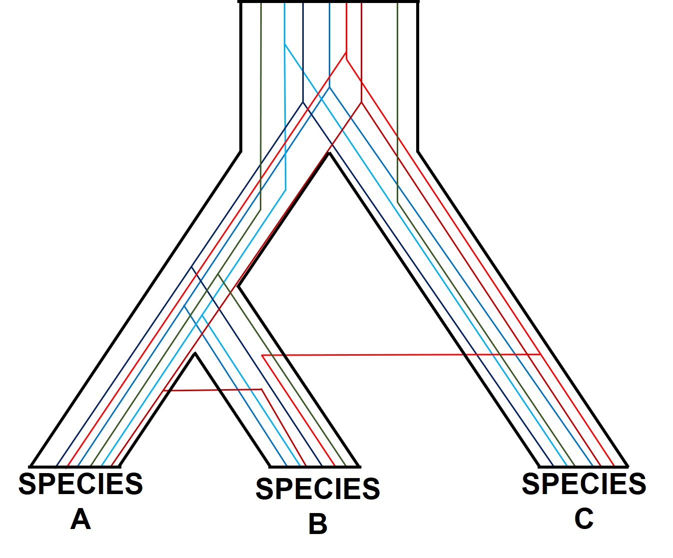
The easiest way to conceptualise gene trees and species trees is to think of individual gene trees that are nested within an overarching species tree. In this sense, individual gene trees can vary from one another (substantially, even) but by looking at the overall trends of many genes we can see how the genome of the species have changed over time.
Gene tree incongruence
Different genes may have different patterns for a number of reasons. Changes in the genetic sequences of organisms over time don’t happen equally across the entire genome, and very specific parts of the genome can evolve in entirely different directions, or at entirely different rates, than the rest of the genome. Let’s take a look at a few ways we could have conflicting gene trees in our studies.
Incomplete lineage sorting
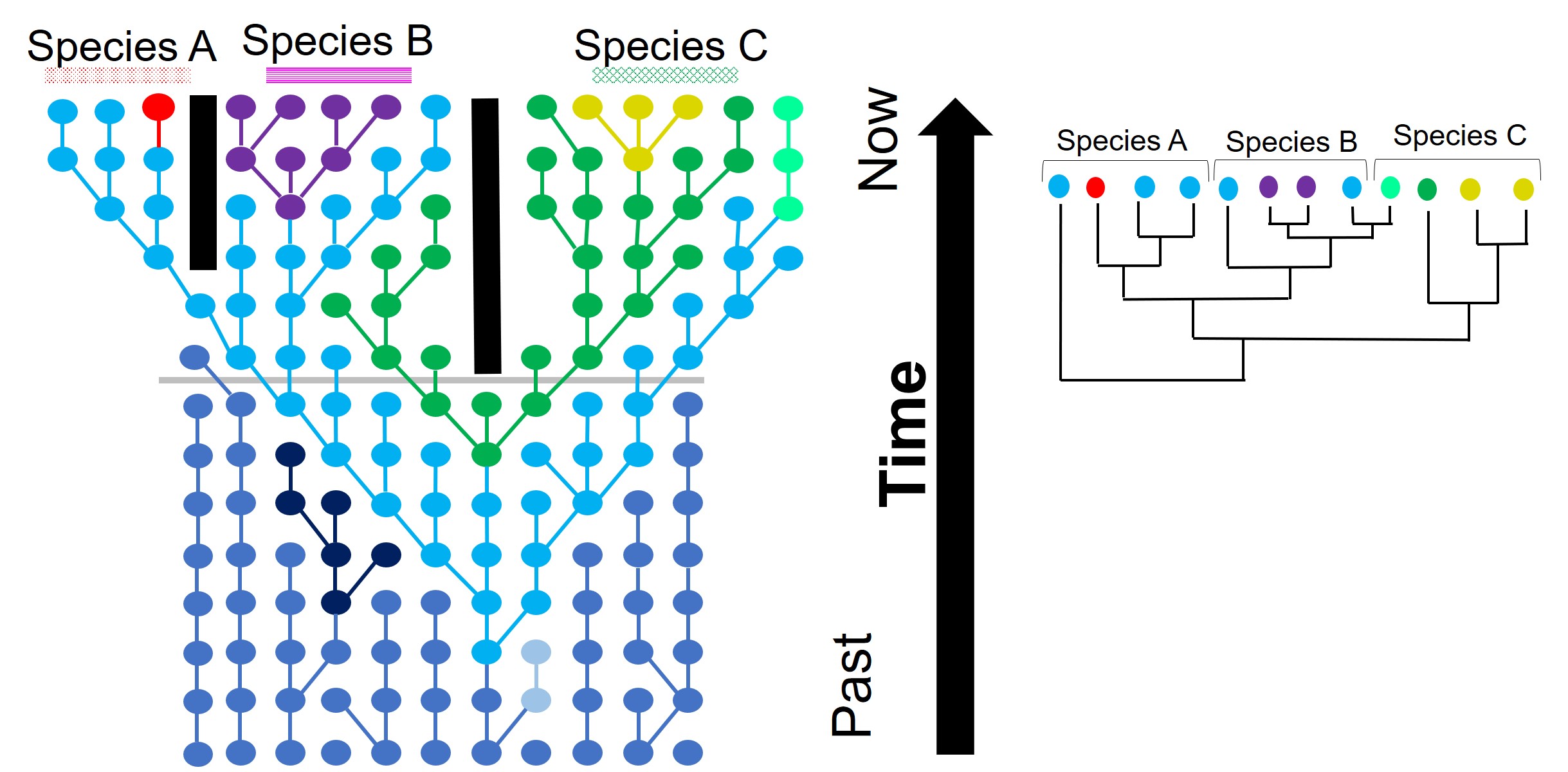
One of the most prolific, but more complicated, ways gene trees can vary from their overarching species tree is due to what we call ‘incomplete lineage sorting’. This is based on the idea that species and the genes that define them are constantly evolving over time, and that because of this different genes are at different stages of divergence between population and species. If we imagine a set of three related populations which have all descended from a single ancestral population, we can start to see how incomplete lineage sorting could occur. Our ancestral population likely has some genetic diversity, containing multiple alleles of the same locus. In a true phylogenetic tree, we would expect these different alleles to ‘sort’ into the different descendent populations, such that one population might have one of the alleles, a second the other, and so on, without them sharing the different alleles between them.
If this separation into new populations has been recent, or if gene flow has occurred between the populations since this event, then we might find that each descendent population has a mixture of the different alleles, and that not enough time has passed to clearly separate the populations. For this to occur, sufficient time for new mutations to occur and genetic drift to push different populations to differently frequent alleles needs to happen: if this is too recent, then it can be hard to accurately distinguish between populations. This can be difficult to interpret (see below figure for a visualisation of this), but there’s a great description of incomplete lineage sorting here.
Hybridisation and horizontal transfer
Another way individual genes may become incongruent with other genes is through another phenomenon we’ve discussed before: hybridisation (or more specifically, introgression). When two individuals from different species breed together to form a ‘hybrid’, they join together what was once two separate gene pools. Thus, the hybrid offspring has (if it’s a first generation hybrid, anyway) 50% of genes from Species A and 50% of genes from Species B. In terms of our phylogenetic analysis, if we picked one gene randomly from the hybrid, we have 50% of picking a gene that reflects the evolutionary history of Species A, and 50% chance of picking a gene that reflects the evolutionary history of Species B. This would change how our outputs look significantly: if we pick a Species A gene, our ‘hybrid’ will look (genetically) very, very similar to Species A. If we pick a Species B gene, our ‘hybrid’ will look like a Species B individual instead. Naturally, this can really stuff up our interpretations of species boundaries, distributions and identities.

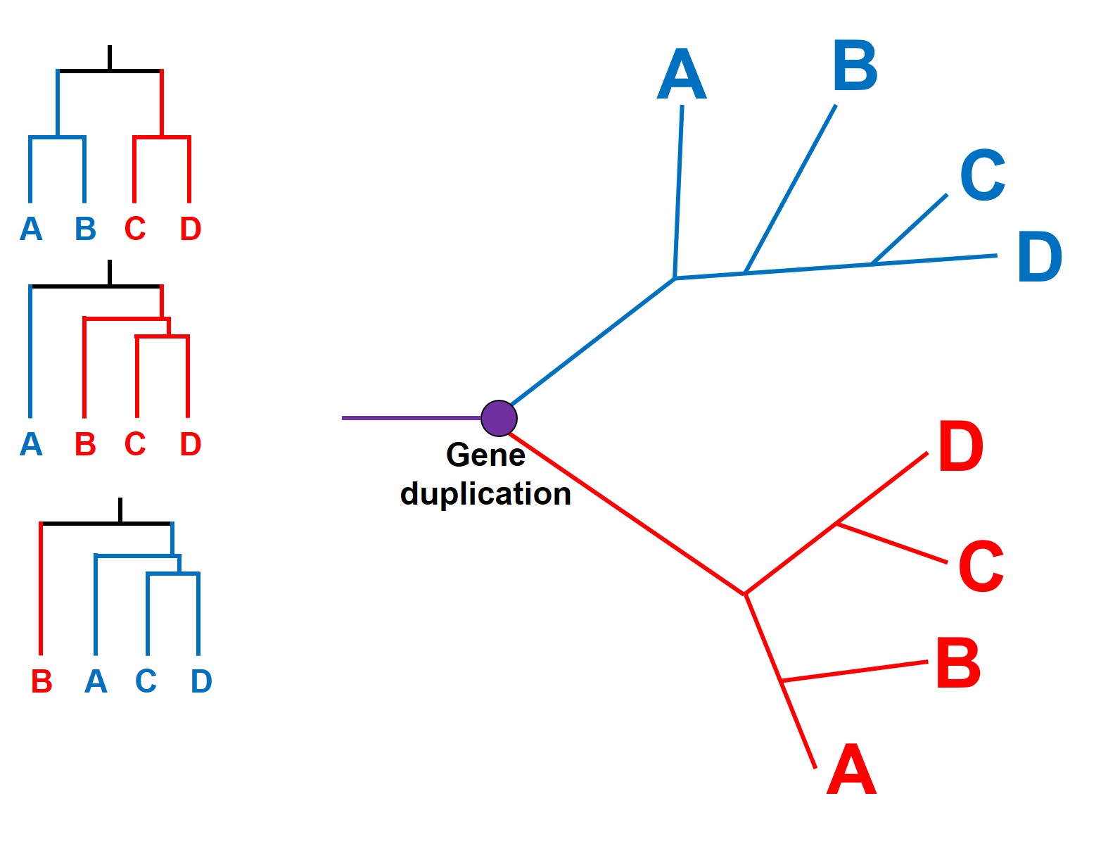
Paralogous genes
More confusingly, we can even have events where a single gene duplicates within a genome. This is relatively rare, although it can have huge effects: for example, salmon have massive genomes as the entire thing was duplicated! Each version of the gene can take on very different forms, functions, and evolve in entirely different ways. We call these duplicated variants paralogous genes: genes that look the same (in terms of sequence), but are totally different genes.
This can have a profound impact as paralogous genes are difficult to detect: if there has been a gene duplication early in the evolutionary history of our phylogenetic tree, then many (or all) of our study samples will have two copies of said gene. Since they look similar in sequence, there’s all possibility that we pick Variant 1 in some species and Variant 2 in other species. Being unable to tell them apart, we can have some very weird and abstract results within our tree. Most importantly, different samples with the same duplicated variant will seem similar to one another (e.g. have evolved from a common ancestor more recently) than it will to any sample of the other variant (even if they came from the exact same species)!
Overcoming incongruence with genomics
Although a tricky conundrum in phylogenetics and evolutionary genetics broadly, gene tree incongruence can largely be overcome with using more loci. As the random changes of any one locus has a smaller effect of the larger total set of loci, the general and broad patterns of evolutionary history can become clearer. Indeed, understanding how many loci are affected by what kind of process can itself become informative: large numbers of introgressed loci can indicate whether hybridisation was recent, strong, or biased towards one species over another, for example. As with many things, the genomic era appears poised to address the many analytical issues and complexities of working with genetic data.
An identity crisis: using genomics to determine species identities
This is the fourth (and final) part of the miniseries on the genetics and process of speciation. To start from Part One, click here.
In last week’s post, we looked at how we can use genetic tools to understand and study the process of speciation, and particularly the transition from populations to species along the speciation continuum. Following on from that, the question of “how many species do I have?” can be further examined using genetic data. Sometimes, it’s entirely necessary to look at this question using genetics (and genomics).
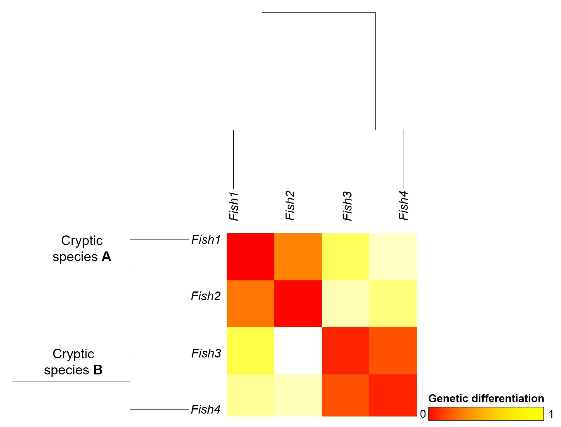
Cryptic species
A concept that I’ve mentioned briefly previously is that of ‘cryptic species’. These are species which are identifiable by their large genetic differences, but appear the same based on morphological, behavioural or ecological characteristics. Cryptic species often arise when a single species has become fragmented into several different populations which have been isolated for a long time from another. Although they may diverge genetically, this doesn’t necessarily always translate to changes in their morphology, ecology or behaviour, particularly if these are strongly selected for under similar environmental conditions. Thus, we need to use genetic methods to be able to detect and understand these species, as well as later classify and describe them.
Genetic tools to study species: the ‘Barcode of Life’
A classically employed method that uses DNA to detect and determine species is referred to as the ‘Barcode of Life’. This uses a very specific fragment of DNA from the mitochondria of the cell: the cytochrome c oxidase I gene, CO1. This gene is made of 648 base pairs and is found pretty well universally: this and the fact that CO1 evolves very slowly make it an ideal candidate for easily testing the identity of new species. Additionally, mitochondrial DNA tends to be a bit more resilient than its nuclear counterpart; thus, small or degraded tissue samples can still be sequenced for CO1, making it amenable to wildlife forensics cases. Generally, two sequences will be considered as belonging to different species if they are certain percentage different from one another.
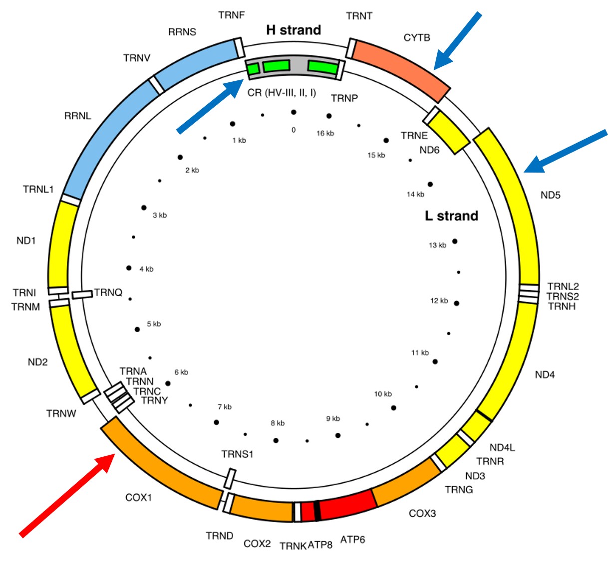
Despite the apparent benefits of CO1, there are of course a few drawbacks. Most of these revolve around the mitochondrial genome itself. Because mitochondria are passed on from mother to offspring (and not at all from the father), it reflects the genetic history of only one sex of the species. Secondly, the actual cut-off for species using CO1 barcoding is highly contentious and possibly not as universal as previously suggested. Levels of sequence divergence of CO1 between species that have been previously determined to be separate (through other means) have varied from anywhere between 2% to 12%. The actual translation of CO1 sequence divergence and species identity is not all that clear.
Gene tree – species tree incongruences
One particularly confounding aspect of defining species based on a single gene, and with using phylogenetic-based methods, is that the history of that gene might not actually be reflective of the history of the species. This can be a little confusing to think about but essentially leads to what we call “gene tree – species tree incongruence”. Different evolutionary events cause different effects on the underlying genetic diversity of a species (or group of species): while these may be predictable from the genetic sequence, different parts of the genome might not be as equally affected by the same exact process.
A classic example of this is hybridisation. If we have two initial species, which then hybridise with one another, we expect our resultant hybrids to be approximately made of 50% Species A DNA and 50% Species B DNA (if this is the first generation of hybrids formed; it gets a little more complicated further down the track). This means that, within the DNA sequence of the hybrid, 50% of it will reflect the history of Species A and the other 50% will reflect the history of Species B, which could differ dramatically. If we randomly sample a single gene in the hybrid, we will have no idea if that gene belongs to the genealogy of Species A or Species B, and thus we might make incorrect inferences about the history of the hybrid species.
There are a number of other processes that could similarly alter our interpretations of evolutionary history based on analysing the genetic make-up of the species. The best way to handle this is simply to sample more genes: this way, the effect of variation of evolutionary history in individual genes is likely to be overpowered by the average over the entire gene pool. We interpret this as a set of individual gene trees contained within a species tree: although one gene might vary from another, the overall picture is clearer when considering all genes together.
Species delimitation
In earlier posts on The G-CAT, I’ve discussed the biogeographical patterns unveiled by my Honours research. Another key component of that paper involved using statistical modelling to determine whether cryptic species were present within the pygmy perches. I didn’t exactly elaborate on that in that section (mostly for simplicity), but this type of analysis is referred to as ‘species delimitation’. To try and simplify complicated analyses, species delimitation methods evaluate possible numbers and combinations of species within a particular dataset and provides a statistical value for which configuration of species is most supported. One program that employs species delimitation is Bayesian Phylogenetics and Phylogeography (BPP): to do this, it uses a plethora of information from the genetics of the individuals within the dataset. These include how long ago the different populations/species separated; which populations/species are most related to one another; and a pre-set minimum number of species (BPP will try to combine these in estimations, but not split them due to computational restraints). This all sounds very complex (and to a degree it is), but this allows the program to give you a statistical value for what is a species and what isn’t based on the genetics and statistical modelling.
The end result of a BPP run is usually reported as a species tree (e.g. a phylogenetic tree describing species relationships) and statistical support for the delimitation of species (0-1 for each species). Because of the way the statistical component of BPP works, it has been found to give extremely high support for species identities. This has been criticised as BPP can, at time, provide high statistical support for genetically isolated lineages (i.e. divergent populations) which are not actually species.
Improving species identities with integrative taxonomy
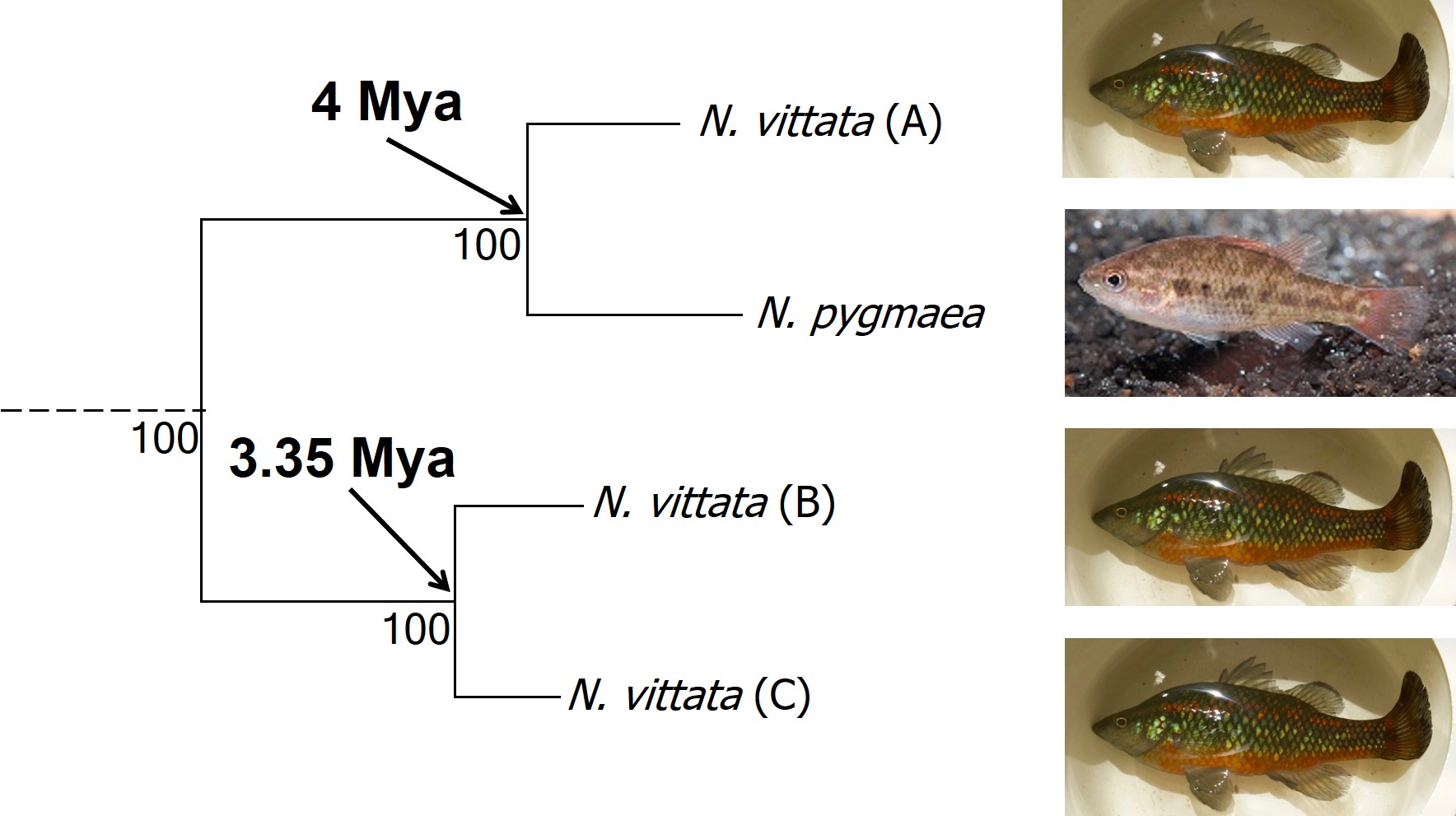
Due to this particular drawback, and the often complex nature of species identity, using solely genetic information such as species delimitation to define species is extremely rare. Instead, we use a combination of different analytical techniques which can include genetic-based evaluations to more robustly assign and describe species. In my own paper example, we suggested that up to three ‘species’ of N. vittata that were determined as cryptic species by BPP could potentially exist pending on further analyses. We did not describe or name any of the species, as this would require a deeper delve into the exact nature and identity of these species.
As genetic data and analytical techniques improve into the future, it seems likely that our ability to detect and determine species boundaries will also improve. However, the additional supported provided by alternative aspects such as ecology, behaviour and morphology will undoubtedly be useful in the progress of taxonomy.
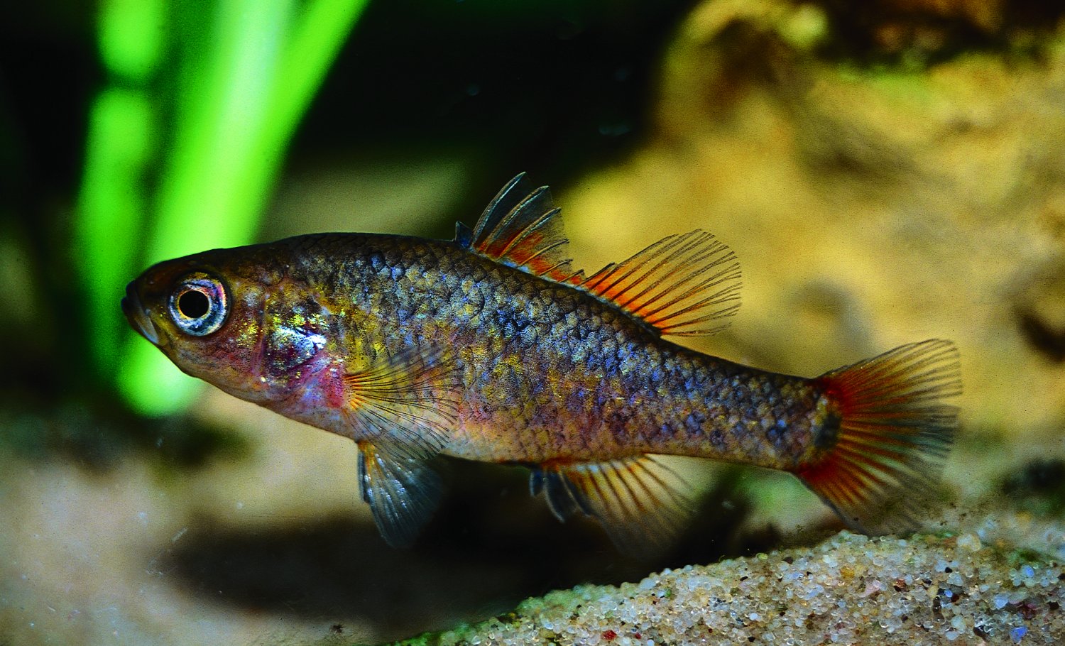
How did pygmy perch swim across the desert?
“Pygmy perch swam across the desert”
As regular readers of The G-CAT are likely aware, my first ever scientific paper was published this week. The paper is largely the results of my Honours research (with some extra analysis tacked on) on the phylogenomics (the same as phylogenetics, but with genomic data) and biogeographic history of a group of small, endemic freshwater fishes known as the pygmy perch. There are a number of different messages in the paper related to biogeography, taxonomy and conservation, and I am really quite proud of the work.
To my honest surprise, the paper has received a decent amount of media attention following its release. Nearly all of these have focused on the biogeographic results and interpretations of the paper, which is arguably the largest component of the paper. In these media releases, the articles are often opened with “…despite the odds, new research has shown how a tiny fish managed to find its way across the arid Australian continent – more than once.” So how did they manage it? These are tiny fish, and there’s a very large desert area right in the middle of Australia, so how did they make it all the way across? And more than once?!
The Great (southern) Southern Land
To understand the results, we first have to take a look at the context for the research question. There are seven officially named species of pygmy perches (‘named’ is an important characteristic here…but we’ll go into the details of that in another post), which are found in the temperate parts of Australia. Of these, three are found with southwest Western Australia, in Australia’s only globally recognised biodiversity hotspot, and the remaining four are found throughout eastern Australia (ranging from eastern South Australia to Tasmania and up to lower Queensland). These two regions are separated by arid desert regions, including the large expanse of the Nullarbor Plain.
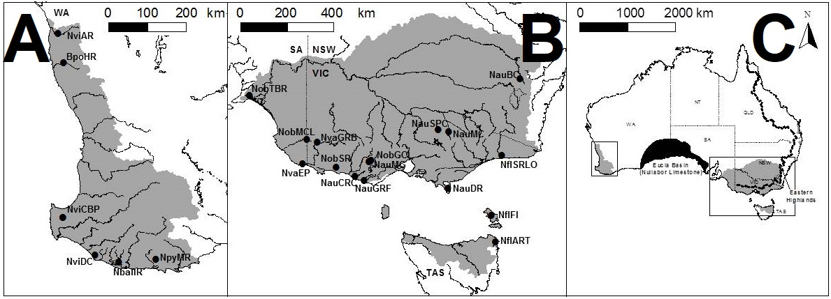
The Nullarbor Plain is a remarkable place. It’s dead flat, has no trees, and most importantly for pygmy perches, it also has no standing water or rivers. The plain was formed from a large limestone block that was pushed up from beneath the Earth approximately 15 million years ago; with the progressive aridification of the continent, this region rapidly lost any standing water drainages that would have connected the east to the west. The remains of water systems from before (dubbed ‘paleodrainages’) can be seen below the surface.

Biogeography of southern Australia
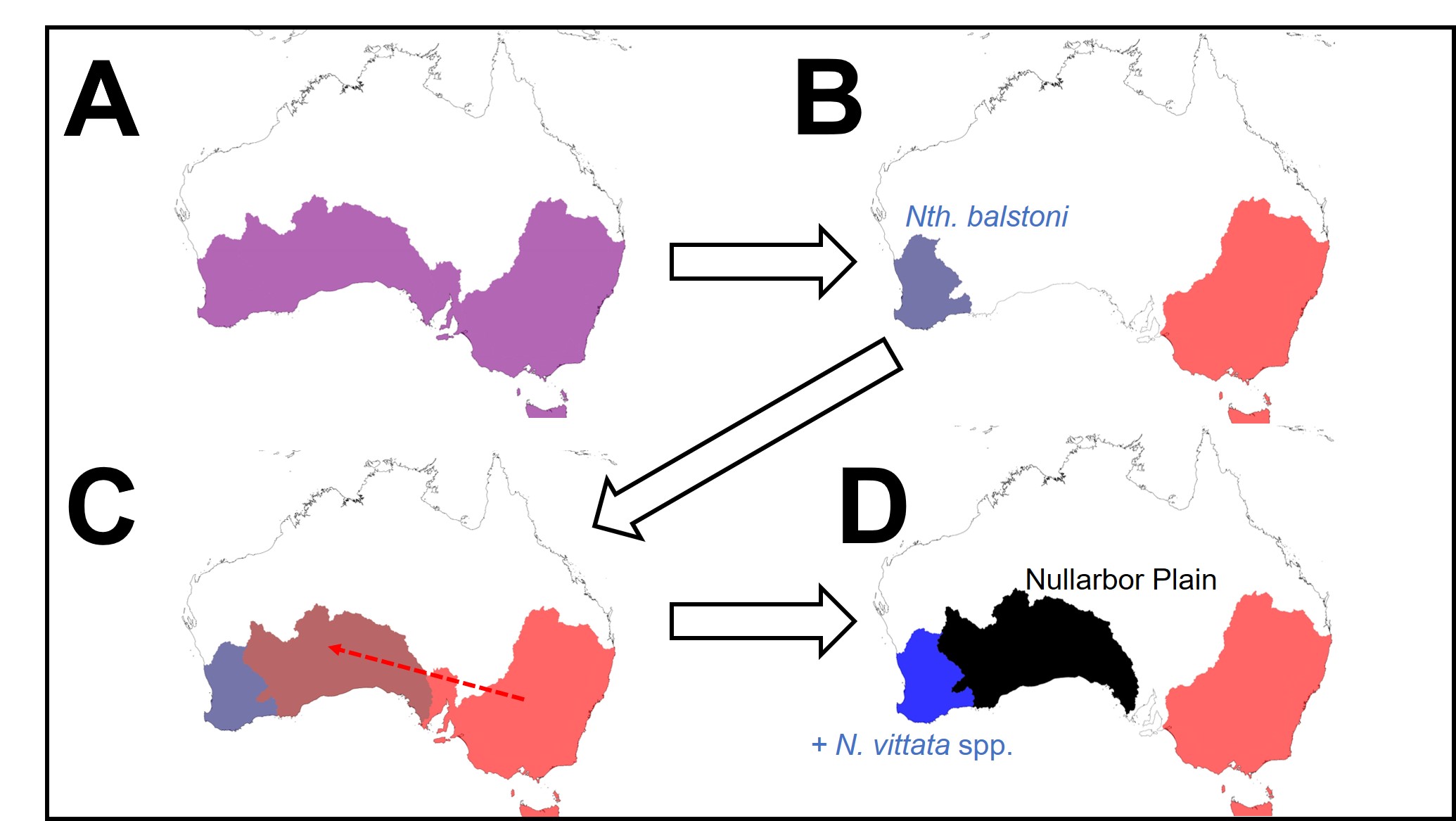
As one might expect, the formation of the Nullarbor Plain was a huge barrier for many species, especially those that depend on regular accessible water for survival. In many species of both plants and animals, we see in their phylogenetic history a clear separation of eastern and western groups around this time; once widely distributed species become fragmented by the plain and diverged from one another. We would most certainly expect this to be true of pygmy perch.
But our questions focus on what happened before the Nullarbor Plain arrived in the picture. More than 15 million years ago, southern Australia was a massively different place. The climate was much colder and wetter, even in central Australia, and we even have records of tropical rainforest habitats spreading all the way down to Victoria. Water-dependent animals would have been able to cross the southern part of the continent relatively freely.
Biogeography of the enigmatic pygmy perches
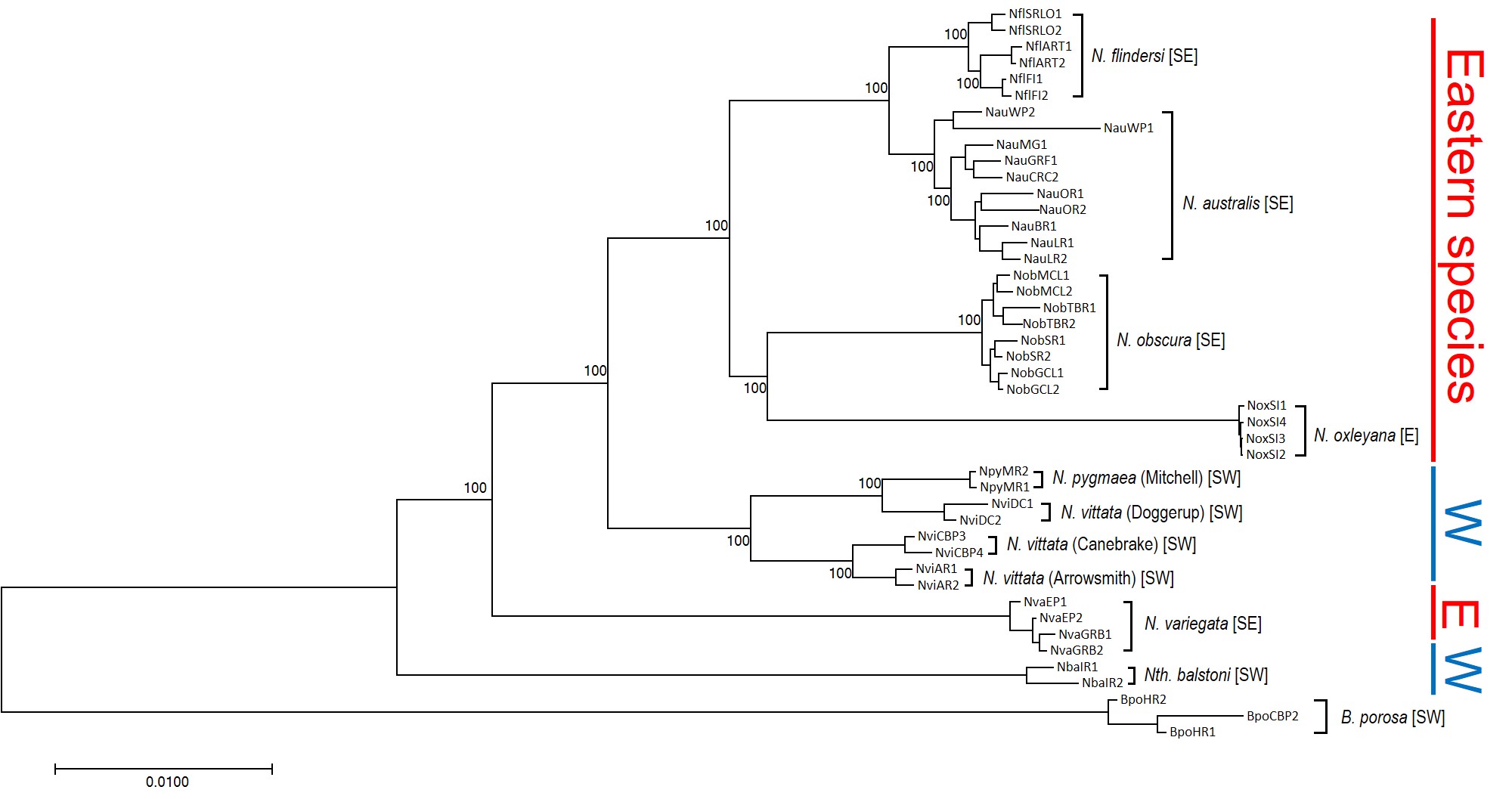
This is where the real difference between everything else and pygmy perch happens. For most species, we see only one east and west split in their phylogenetic tree, associated with the Nullarbor Plain; before that, their ancestors were likely distributed across the entire southern continent and were one continuous unit.
Not for pygmy perch, though. Our phylogenetic patterns show that there were multiple splits between eastern and western ancestral pygmy perch. We can see this visually within the phylogenetic tree; some western species of pygmy perches are more closely related, from an evolutionary perspective, to eastern species of pygmy perches than they are to other western species. This could imply a couple different things; either some species came about by migration from east to west (or vice versa), and that this happened at least twice, or that two different ancestral pygmy perches were distributed across all of southern Australia and each split east-west at some point in time. These two hypotheses are called “multiple invasion” and “geographic paralogy”, respectively.
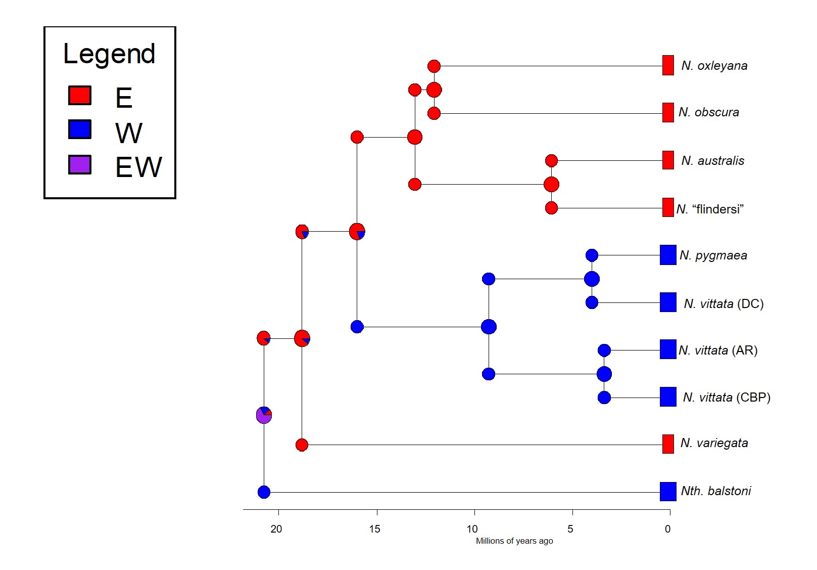
So, which is it? We delved deeper into this using a type of analysis called ‘ancestral clade reconstruction’. This tries to guess the likely distributions of species ancestors using different models and statistical analysis. Our results found that the earliest east-west split was due to the fragmentation of a widespread ancestor ~20 million years ago, and a migration event facilitated by changing waterways from the Nullarbor Plain pushing some eastern pygmy perches to the west to form the second group of western species. We argue for more than one migration across Australia since the initial ancestor of pygmy perches must have expanded from some point (either east or west) to encompass the entirety of southern Australia.
So why do we see this for pygmy perch and no other species? Well, that’s the real mystery; out of all of the aquatic species found in southeast and southwest Australia, pygmy perch are one of the worst at migrating. They’re very picky about habitat, small, and don’t often migrate far unless pushed (by, say, a flood). It is possible that unrecorded extinct species of pygmy perch might help to clarify this a little, but the chances of finding a preserved fish fossil (let alone for a fish less than 8cm in size!) is extremely unlikely. We can really only theorise about how they managed to migrate.
What does this mean for pygmy perches?
Nearly all species of pygmy perch are threatened or worse in the conservation legislation; there have been many conservation efforts to try and save the worst-off species from extinction. Pygmy perches provide a unique insight to the history of the Australian climate and may be a key in unlocking some of the mysteries of what our land was like so long ago. Every species is important for conservation and even those small, hard-to-notice creatures that we might forget about play a role in our environmental history.
The direction of evolution: divergence vs. convergence
Direction of evolution
We’ve talked previously on The G-CAT about how the genetic underpinning of certain evolutionary traits can change in different directions depending on the selective pressure it is under. Particularly, we can see how the frequency of different alleles might change in one direction or another, or stabilise somewhere in the middle, depending on its encoded trait. But thinking bigger picture than just the genetics of one trait, we can actually see that evolution as an entire process works rather similarly.
Divergent evolution
The classic view of the direction of evolution is based on divergent evolution. This is simply the idea that a particular species possess some ancestral trait. The species (or population) then splits into two (for one reason or another), and each one of these resultant species and populations evolves in a different way to the other. Over time, this means that their traits are changing in different directions, but ultimately originate from the same ancestral source.
Evidence for divergent evolution is rife throughout nature, and is a fundamental component of all of our understanding of evolution. Divergent evolution means that, by comparing similar traits in two species (called homologous traits), we can trace back species histories to common ancestors. Some impressive examples of this exist in nature, such as the number of bones in most mammalian species. Humans have the same number of neck bones as giraffes; thus, we can suggest that the ancestor of both species (and all mammals) probably had a similar number of neck bones. It’s just that the giraffe lineage evolved longer bones whereas other lineages did not.

Convergent evolution
But of course, evolution never works as simply as you want it to, and sometimes we can get the direct opposite pattern. This is called convergent evolution, and occurs when two completely different species independently evolve very similar (sometimes practically identical) traits. This is often caused by a limitation of the environment; some extreme demand of the environment requires a particular physiological solution, and thus all species must develop that trait in order to survive. An example of this would be the physiology of carnivorous marsupials like Tasmanian devils or thylacines: despite being in another Class, their body shapes closely resemble something more canid. Likely, the carnivorous diet places some constraints on physiology, particularly jaw structure and strength.

A more dramatic (and potentially obvious) example of convergent evolution would be wings and the power of flight. Despite the fact that butterflies, bees, birds and bats all have wings and can fly, most of them are pretty unrelated to one another. It seems much more likely that flight evolved independently multiple times, rather than the other 99% of species that shared the same ancestor lost the capacity of flight.
Parallel evolution
Sometimes convergent evolution can work between two species that are pretty closely related, but still evolved independently of one another. This is distinguished from other categories of evolution as parallel evolution: the main difference is that while both species may have shared the same start and end point, evolution has acted on each one independent of the other. This can make it very difficult to diagnose from convergent evolution, and is usually determined by the exact history of the trait in question.
Parallel evolution is an interesting field of research for a few reasons. Firstly, it provides a scenario in which we can more rigorously test expectations and outcomes of evolution in a particular environment. For example, if we find traits that are parallel in a whole bunch of fish species in a particular region, we can start to look at how that particular environment drives evolution across all fish species, as opposed to one species case studies.
Following from that logic, it is then important to question the mechanisms of parallelism. From a genetic point of view, do these various species use the same genes (and genetic variants) to produce the same identical trait? Or are there many solutions to the selective question in nature? While these questions are rather complicated, and there has been plenty of evidence both for and against parallel genetic underpinning of parallel traits, it seems surprisingly often that many different genetic combinations can be used to get the same result. This gives interesting insight into how complex genetic coding of traits can be, and how creative and diverse evolution can be in the real world.
Where is evolution going?

So, where is evolution going for nature? Well, the answer is probably all over the place, but steered by the current environmental circumstances. Predicting the evolutionary impacts of particular environmental change (e.g. climate change) is exceedingly difficult but a critical component of understanding the process of evolution and the future of species. Evolution continually surprises us with creative solution to complex problems and I have no doubt new mysteries will continue to be thrown at us as we delve deeper.
