It should come as no surprise to any reader of The G-CAT that I’m a firm believer against the false dichotomy (and yes, I really do love that phrase) of “nature versus nurture.” Primarily, this is because the phrase gives the impression of some kind of counteracting balance between intrinsic (i.e. usually genetic) and extrinsic (i.e. usually environmental) factors and how they play a role in behaviour, ecology and evolution. While both are undoubtedly critical for adaptation by natural selection, posing this as a black-and-white split removes the possibility of interactive traits.
The real Circle of Life. Not only do genes and the environment interact with one another, but genes may interact with other genes and environments may be complex and multi-faceted.
A very simplified example of adaptation from genetic variation. In this example, we have two different alleles of a single gene (orange and blue). Natural selection favours the blue allele so over time it increases in frequency. The difference between these two alleles is at least one base pair of DNA sequence; this often arises by mutation processes.
Despite how important the underlying genes are for the formation of proteins and definition of physiology, they are not omnipotent in that regard. In fact, many other factors can influence how genetic traits relate to phenotypic traits: we’ve discussed a number of these in minor detail previously. An example includes interactions across different genes: these can be due to physiological traits encoded by the cumulative presence and nature of many loci (as in quantitative trait loci and polygenic adaptation). Alternatively, one gene may translate to multiple different physiological characters if it shows pleiotropy.
Differential expression
One non-direct way genetic information can impact on the phenotype of an organism is through something we’ve briefly discussed before known as differential expression. This is based on the notion that different environmental pressures may affect the expression (that is, how a gene is translated into a protein) in alternative ways. This is a fundamental underpinning of what we call phenotypic plasticity: the concept that despite having the exact same (or very similar) genes and alleles, two clonal individuals can vary in different traits. The is related to the example of genetically-identical twins which are not necessarily physically identical; this could be due to environmental constraints on growth, behaviour or personality.
An example of differential expression in wild populations of southern pygmy perch, courtesy of Brauer et al. (2017). In this figure, each column represents a single individual fish, with the phylogenetic tree and coloured boxes at the top indicating the different populations. Each row represents a different gene (this is a subset of 50 from a much larger dataset). The colour of each cell indicates whether the expression of that gene is expressed more (red) or less (blue) than average. As you can see, the different populations can clearly be seen within their expression profiles, with certain genes expressing more or less in certain populations.
The discovery of epigenetic markers and their influence on gene expression has opened up the possibility of understanding heritable traits which don’t appear to be clearly determined by genetics alone. For example, research into epigenetics suggest that heritable major depressive disorder (MDD) may be controlled by the expression of genes, rather than from specific alleles or genetic variants themselves. This is likely true for a number of traits for which the association to genotype is not entirely clear.
Epigenetic adaptation?
From an evolutionary standpoint again, epigenetics can similarly influence the ‘bang for a buck’ of particular genes. Being able to translate a single gene into many different forms, and for this to be linked to environmental conditions, allows organisms to adapt to a variety of new circumstances without the need for specific adaptive genes to be available. Following this logic, epigenetic variation might be critically important for species with naturally (or unnaturally) low genetic diversity to adapt into the future and survive in an ever-changing world. Thus, epigenetic information might paint a more optimistic outlook for the future: although genetic variation is, without a doubt, one of the most fundamental aspects of adaptability, even horrendously genetically depleted populations and species might still be able to be saved with the right epigenetic diversity.
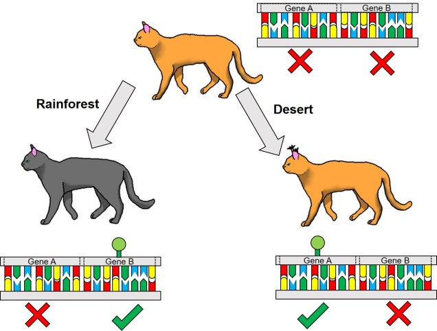
A relatively simplified example of adaptation from epigenetic variation. In this example, we have a species of cat; the ‘default’ cat has non-tufted ears and an orange coat. These two traits are controlled by the expression of Genes A and B, respectively: in the top cat, neither gene is expressed. However, when this cat is placed into different environments, the different genes are “switched on” by epigenetic factors (the green markers). In a rainforest environment, the dark foliage makes darker coat colour more adaptive; switching on Gene B allows this to happen. Conversely, in a desert environment switching on Gene A causes the cat to develop tufts on its ears, which makes it more effective at hunting prey hiding in the sands. Note that in both circumstances, the underlying genetic sequence (indicated by the colours in the DNA) is identical: only the expression of those genes change.
Epigenetic research, especially from an ecological/evolutionary perspective, is a very new field. Our understanding of how epigenetic factors translate into adaptability, the relative performance of epigenetic vs. genetic diversity in driving adaptability, and how limited heritability plays a role in adaptation is currently limited. As with many avenues of research, further studies in different contexts, experiments and scopes will reveal further this exciting new aspect of evolutionary and conservation genetics. In short: watch this space! And remember, ‘nature is nurture’ (and vice versa)!
A number of timesbefore on The G-CAT, we’ve discussed the idea of using the frequency of different genetic variants (alleles) within a particular population or species to test a number of different questions about evolution, ecology and conservation. These are all based on the central notion that certain forces of nature will alter the distribution and frequency of alleles within and across populations, and that these patterns are somewhat predictable in how they change.
One particular distinction we need to make early here is the difference between allele frequency and allele identity. In these analyses, often we are working with the same alleles (i.e. particular variants) across our populations, it’s just that each of these populations may possess these particular alleles in different frequencies. For example, one population may have an allele (let’s call it Allele A) very rarely – maybe only 10% of individuals in that population possess it – but in another population it’s very common and perhaps 80% of individuals have it. This is a different level of differentiation than comparing how different alleles mutate (as in the coalescent) or how these mutations accumulate over time (like in many phylogenetic-based analyses).
An example of the difference between allele frequency and identity.In this example (and many of the figures that follow in this post), the circle denote different populations, within which there are individuals which possess either an A gene (blue) or a B gene. Left: If we compared Populations 1 and 2, we can see that they both have A and B alleles. However, these alleles vary in their frequency within each population, with an equal balance of A and B in Pop 1 and a much higher frequency of B in Pop 2. Right: However, when we compared Pop 3 and 4, we can see that not only do they vary in frequencies, they vary in the presence of alleles, with one allele in each population but not the other.
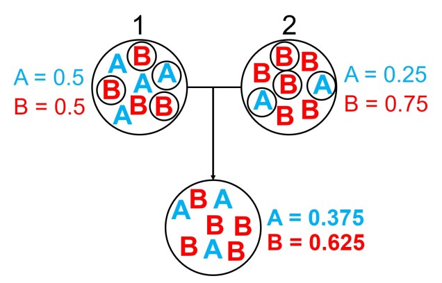
An example of how gene flow across populations homogenises allele frequencies. We start with two initial populations (1 and 2 from above), which have very different allele frequencies. Hybridising individuals across the two populations means some alleles move from Pop 1 and Pop 2 into the hybrid population: which alleles moves is random (the smaller circles). Because of this, the resultant hybrid population has an allele frequency somewhere in between the two source populations: think of like mixing red and blue cordial and getting a purple drink.
An example of a Structure plot which long-term The G-CAT readers may be familiar with. This is taken from Brauer et al. (2013), where the authors studied the population structure of the Yarra pygmy perch. Each small column represents a single individual, with the colours representing how well the alleles of that individual fit a particular genetic population (each population has one colour). The numbers and broader columns refer to different ‘localities’ (different from populations) where individuals were sourced. This shows clear strong population structure across the 4 main groups, except for in Locality 6 where there is a mixture of Eastern and Merri/Curdies alleles.
Determining genetic bottlenecks and demographic change
A diagram of how allele frequencies change in genetic bottlenecks due to genetic drift. Left: Large circles again denote a population (although across different sequential times), with smaller circle denoting which alleles survive into the next generation (indicated by the coloured arrows). We start with an initial ‘large’ population of 8, which is reduced down to 4 and 2 in respective future times. Each time the population contracts, only a select number of alleles (or individuals) ‘survive’: assuming no natural selection is in process, this is totally random from the available gene pool. Right: We can see that over time, the frequencies of alleles A and B shift dramatically, leading to the ‘extinction’ of Allele B due to genetic drift. This is because it is the less frequent allele of the two, and in the smaller population size has much less chance of randomly ‘surviving’ the purge of the genetic bottleneck.
An example of how the frequency of alleles might vary under natural selection in correlation to the environment. In this example, the blue allele A is adaptive and under positive selection in the more intense environment, and thus increases in frequency at higher values. Contrastingly, the red allele B is maladaptive in these environments and decreases in frequency. For comparison, the black allele shows how the frequency of a neutral (non-adaptive or maladaptive) allele doesn’t vary with the environment, as it plays no role in natural selection.
Fixed differences are sometimes used as a type of diagnostic trait for species. This means that each ‘species’ has genetic variants that are not shared at all with its closest relative species, and that these variants are so strongly under selection that there is no diversity at those loci. Often, fixed differences are considered a level above populations that differ by allelic frequency only as these alleles are considered ‘diagnostic’ for each species.
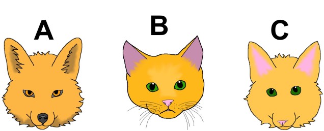
An example of the difference between fixed differences and allelic frequency differences. In this example, we have 5 cats from 3 different species, sequencing a particular target gene. Within this gene, there are three possible alleles: T, A or G respectively. You’ll quickly notice that the T allele is both unique to Species A and is present in all cats of that species (i.e. is fixed). This is a fixed difference between Species A and the other two. Alleles A and G, however, are present in both Species B and C, and thus are not fixed differences even if they have different frequencies.
To distinguish between the two, we often use the overall frequency of alleles in a population as a basis for determining how likely two individuals share an allele by random chance. If alleles which are relatively rare in the overall population are shared by two individuals, we expect that this similarity is due to family structure rather than population history. By factoring this into our relatedness estimates we can get a more accurate overview of how likely two individuals are to be related using genetic information.
The wild world of allele frequency
Despite appearances, this is just a brief foray into the many applications of allele frequency data in evolution, ecology and conservation studies. There are a plethora of different programs and methods that can utilise this information to address a variety of scientific questions and refine our investigations.
This is Part 1 of a four part miniseries on the process of speciation; how we get new species, how we can see this in action, and the end results of the process. This week, we’ll start with a seemingly obvious question: what is a species?
The definition of a ‘species’
‘Species’ are a human definition of the diversity of life. When we talk about the diversity of life, and the myriad of creatures and plants on Earth, we often talk about species diversity. This might seem glaringly obvious, but there’s one key issue: what is a species, anyway? While we might like to think of them as discrete and obvious groups (a dog is definitely not the same species as a cat, for example), the concept of a singular “species” is actually the result of human categorisation.
In reality, the diversity of life is spread across a huge spectrum of differentiation: from things which are closely related but still different to us (like chimps), to more different again (other mammals), to hardly relatable at all (bacteria and plants). So, what is the cut-off for calling something a species, and not a different genus, family, or kingdom? Or alternatively, at what point do we call a specific sub-group of a species as a sub-species, or another species entirely?
This might seem like a simple question: we look at two things, and they look different, so they must be different species, right? Well, of course, nature is never simple, and the line between “different” and “not different” is very blurry. Here’s an example: consider that you knew nothing about the history, behaviour or genetics of dogs. If you simply looked at all the different breeds of dogs on Earth, you might suggest that there are hundreds of species of domestic dogs. That seems a little excessive though, right? In fact, the domestic dog, Eurasian wolf, and the Australian dingo are all the same species (but different subspecies, along with about 38 others…but that’s another issue altogether).
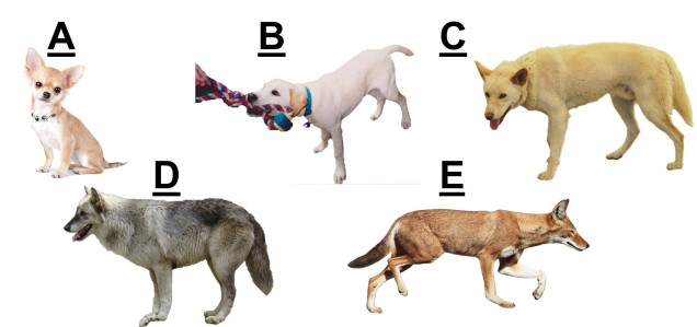
Morphology can be misleading for identifying species. In this example, we have A) a dog, B) also a dog, C) still a dog, D) yet another dog, and E) not a dog. For the record, A-D are all Canis lupus of some variety; A and B are domestic dogs (Canis lupus familiaris), C is a dingo (Canis lupus dingo) and D is a grey wolf (Canis lupus lupus). E, however, isthe Ethiopian wolf, Canis simensis.
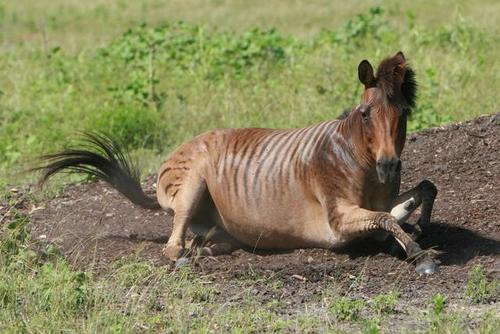
For example, a horse and zebra can breed to produce a zorse, however zorse are fundamentally infertile (due to the different number of chromosomes between a horse and a zebra) and thus a horse is a different species to a zebra. However, a German Shepherd and a chihuahua can breed and make a hybrid mutt, so they are the same species.
A zorse, which shows its hybrid nature through zebra stripes and horse colouring. These two are still separate species since zorses are infertile, and thus are not a singular stable entity.
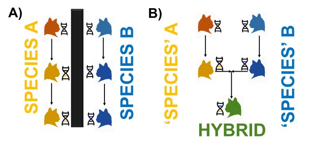
An example of how reproductive isolation maintains genetic and evolutionary independence of species. In A), our cat groups are robust species, reproductively isolated from one another (as shown by the black box). When each species undergoes natural selection and their genetic variation changes (colour changes on the cats and DNA), these changes are kept within each lineage. This contrasts to B), where genetic changes can be transferred between species. Without reproductive isolation, evolution in the orange lineage and the blue lineage can combine within hybrids, sharing the evolutionary pathways of both ancestral species.
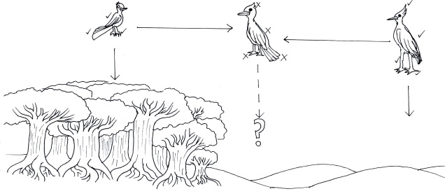
An example of unfit hybrids causing effective reproductive isolation. In this example, we have two different bird species adapted to very different habitats; a smaller, long-tailed bird (left) adapted to moving through dense forest, and a large, longer-legged bird (right) adapted to traversing arid deserts. When (or if) these two species hybridised, the resultant offspring would be middle of the road, possessing too few traits to be adaptive in either the forest or the desert and no fitting intermediate environment available. Measuring exactly how unfit this hybrid would be is a difficult task in establishing species boundaries.
Integrative taxonomy
To try and account for the issues with the BSC, taxonomists try to push for the usage of “integrative taxonomy”. This means that species should be defined by multiple different agreeing concepts, such as reproductive isolation, genetic differentiation, behavioural differences, and/or ecological traits. The more traits that can separate the two, the greater support there is for the species to be separated: if they disagree, then more information is needed to determine exactly whether or not that should be called different species. Debates about taxonomy are ongoing and are likely going to be relevant for years to come, but form critical components of understanding biodiversity, patterns of evolution, and creating effective conservation legislation to protect endangered or threatened species (for whichever groups we decide are species).