For anyone who has had to study geography at some point in their education, you’d likely be familiar with the idea of river courses drawn on a map. They’re so important, in fact, that they are often the delimiting factor in the edges of countries, states or other political units. Water is a fundamental requirement of all forms of life and the riverways that scatter the globe underpin the maintenance, structure and accumulation of a large swathe of biodiversity.
Australia is renowned for its unique diversity of species, and likewise for the diversity of ecosystems across the island continent. Although many would typically associate Australia with the golden sandy beaches, palm trees and warm weather of the tropical east coast, other ecosystems also hold both beautiful and interesting characteristics. Even the regions that might typically seem the dullest – the temperate zones in the southern portion of the continent – themselves hold unique stories of the bizarre and wonderful environmental history of Australia.
The two temperate zones
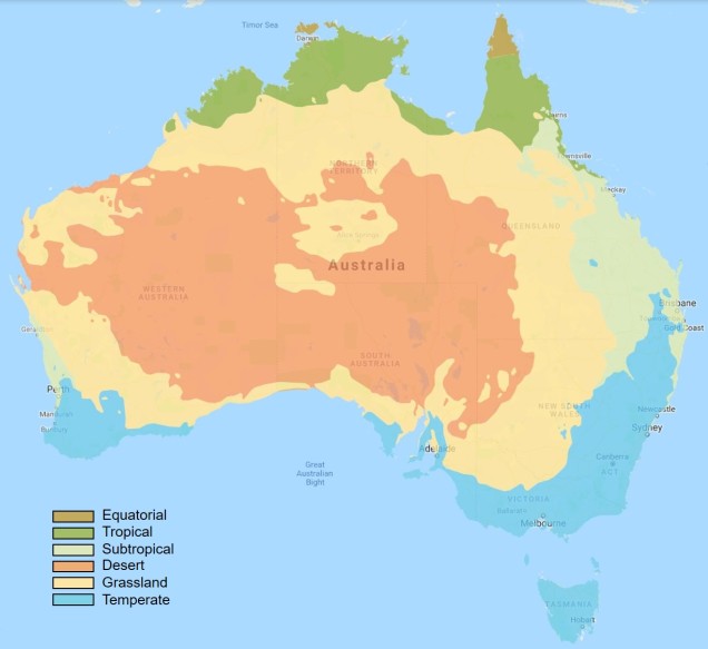
Within Australia, the temperate zone is actually separated into two very distinct and separate regions. In the far south-western corner of the continent is the southwest Western Australia temperate zone, which spans a significant portion. In the southern eastern corner, the unnamed temperate zone spans from the region surrounding Adelaide at its westernmost point, expanding to the east and encompassing Tasmanian and Victoria before shifting northward into NSW. This temperate zones gradually develops into the sub-tropical and tropical climates of more northern latitudes in Queensland and across to Darwin.
The climatic classification (Koppen-Geiger) of Australia’s ecosystems, derived from the Atlas of Living Australia. The light blue region highlights the temperate zones discussed here, with an isolated region in the SW and the broader region of the SE as it transitions into subtropical and tropical climates northward.
The divide separating these two regions might be familiar to some readers – the Nullarbor Plain. Not just a particularly good location for fossils and mineral ores, the Nullarbor Plain is an almost perfectly flat arid expanse that stretches from the western edge of South Australia to the temperate zone of the southwest. As the name suggests, the plain is totally devoid of any significant forestry, owing to the lack of available water on the surface. This plain is a relatively ancient geological structure, and finished forming somewhere between 14 and 16 million years ago when tectonic uplift pushed a large limestone block upwards to the surface of the crust, forming an effective drain for standing water with the aridification of the continent. Thus, despite being relatively similar bioclimatically, the two temperate zones of Australia have been disconnected for ages and boast very different histories and biota.
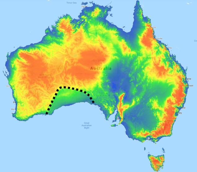
A map of elevation across the Australian continent, also derived from the Atlas of Living Australia. The dashed black line roughly outlines the extent of the Nullarbor Plain, a massively flat arid expanse.
The hotspot of the southwest
The southwest temperate zone – commonly referred to as southwest Western Australia (SWWA) – is an island-like bioregion. Isolated from the rest of the temperate Australia, it is remarkably geologically simple, with little topographic variation (only the Darling Scarp that separates the lower coast from the higher elevation of the Darling Plateau), generally minor river systems and low levels of soil nutrients. One key factor determining complexity in the SWWA environment is the isolation of high rainfall habitats within the broader temperate region – think of islands with an island.
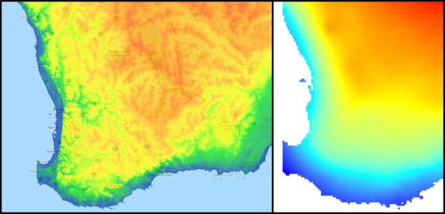
A figure demonstrating the environmental characteristics of SWWA, using data from the Atlas of Living Australia. Left: An elevation map of the region, showing some mountainous variation, but only one significant steep change along the coast (blue area). Right: A summary of 19 different temperature and precipitation variables, showing a relatively weak gradient as the region shifts inland.
Despite the lack of geological complexity and the perceived diversity of the tropics, the temperate zone of SWWA is the only internationally recognisedbiodiversity hotspot within Australia. As an example, SWWA is inhabited by ~7,000 different plant species, half of which are endemic to the region. Not to discredit the impressive diversity of the rest of the continent, of course. So why does this area have even higher levels of species diversity and endemism than the rest of mainland Australia?
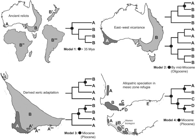
A demonstration of some of the different patterns which might explain the high biodiversity of SWWA, from Rix et al. (2015). These predominantly relate to different biogeographic mechanisms that might have driven diversification in the region, from survivors of the Gondwana era to the more recent fragmentation of mesic habitats.
Well, a number of factors may play significant roles in determining this. One of these is the ancient and isolated nature of the region: SWWA has been separated from the rest of Australia for at least 14 million years, with many species likely originating much earlier than this. Because of this isolation, species occurring within SWWA have been allowed to undergo adaptive divergence from their east coast relatives, forming unique evolutionary lineages. Furthermore, the southwest corner of the continent was one of the last to break away from Antarctica in the dismantling of Gondwana >30 million years ago. Within the region more generally, isolation of mesic (wetter) habitats from the broader, arid (xeric) habitats also likely drove the formation of new species as distributions became fragmented or as species adapted to the new, encroaching xeric habitat. Together, this varies mechanisms all likely contributed in some way to the overall diversity of the region.
The temperate south-east of Australia
Contrastingly, the temperate region in the south-east of the continent is much more complex. For one, the topography of the zone is much more variable: there are a number of prominent mountain chains (such as the extended Great Dividing Range), lowland basins (such as the expansive Murray-Darling Basin) and variable valley and river systems. Similarly, the climate varies significantly within this temperate region, with the more northern parts featuring more subtropical climatic conditions with wetter and hotter summers than the southern end. There is also a general trend of increasing rainfall and lower temperatures along the highlands of the southeast portion of the region, and dry, semi-arid conditions in the western lowland region.
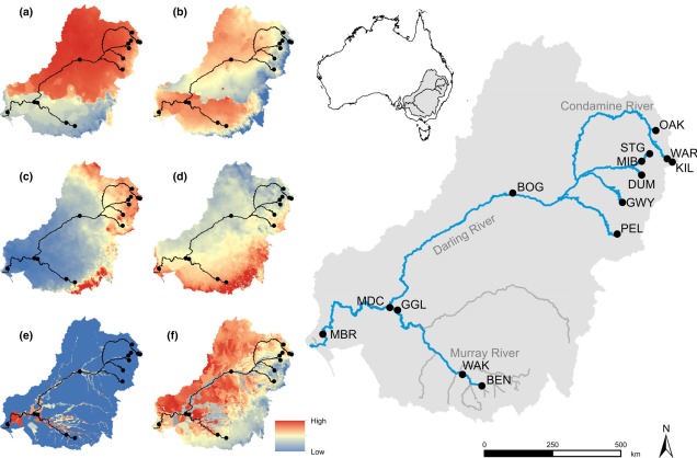
A map demonstrating the climatic variability across the Murray-Darling Basin (which makes up a large section of the SE temperate zone), from Brauer et al. (2018). The different heat maps on the left describe different types of variables; a) and b) represent temperature variables, c) and d) represent precipitation (rainfall) variables, and e) and f) represent water flow variables. Each variable is a summary of a different set of variables, hence the differences.
A complicated history
The south-east temperate zone is not only variable now, but has undergone some drastic environmental changes over history. Massive shifts in geology, climate and sea-levels have particularly altered the nature of the area. Even volcanic events have been present at some time in the past.
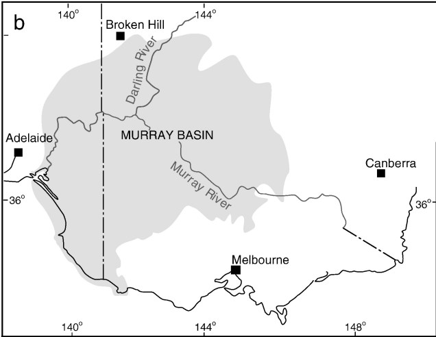
One key hydrological shift that massively altered the region was the paleo-megalake Bungunnia. Not just a list of adjectives, Bungunnia was exactly as it’s described: a historically massive lake that spread across a huge area prior to its demise ~1-2 million years ago. At its largest size, Lake Bungunnia reached an area of over 50,000 km2, spreading from its westernmost point near the current Murray mouth although to halfway across Victoria. Initially forming due to a tectonic uplift event along the coastal edge of the Murray-Darling Basin ~3.2 million years ago, damming the ancestral Murray River (which historically outlet into the ocean much further east than today). Over the next few million years, the size of the lake fluctuated significantly with climatic conditions, with wetter periods causing the lake to overfill and burst its bank. With every burst, the lake shrank in size, until a final break ~700,000 years ago when the ‘dam’ broke and the full lake drained.
A map demonstrating the sheer size of paleo megalake Bungunnia at it’s largest extent, taken from McLaren et al. (2012).
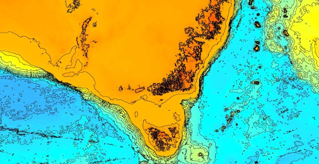
Another change in the historic environment readers may be more familiar with is the land-bridge that used to connect Tasmania to the mainland. Dubbed the Bassian Isthmus, this land-bridge appeared at various points in history of reduced sea-levels (i.e. during glacial periods in Pleistocene cycle), predominantly connecting via the still-above-water Flinders and Cape Barren Islands. However, at lower sea-levels, the land bridge spread as far west as King Island: central to this block of land was a large lake dubbed the Bass Lake (creative). The Bassian Isthmus played a critical role in the migration of many of the native fauna of Tasmania (likely including the Indigenous peoples of the now-island), and its submergence and isolation leads to some distinctive differences between Tasmanian and mainland biota. Today, the historic presence of the Bassian Isthmus has left a distinctive mark on the genetic make-up of many species native to the southeast of Australia, including dolphins, frogs, freshwater fishes and invertebrates.
An elevation (Etopo1) map demonstrating the now-underwater land bridge between Tasmania and the mainland. Orange colours denote higher areas whilst light blue represents lower sections.
Don’t underestimate the temperates
Although tropical regions get most of the hype for being hotspots of biodiversity, the temperate zones of Australia similarly boast high diversity, unique species and document a complex environmental history. Studying how the biota and environment of the temperate regions has changed over millennia is critical to predicting the future effects of climatic change across large ecosystems.
Typically, the maximum distribution of species is based on their ecological tolerances: that is, the most extreme environments they can tolerate and proliferate within. Of course, there are a huge number of other factors on top of just natural environment which can shape species distributions, particularly related to human-induced environmental changes (or introducing new species as invasive pests, which we seem to be good at). But exactly where species are and why they occur there are intrinsically linked to the adaptive characteristics of species relative to their environment.
The generalised pipeline of SDM, taken from Svenning et al. (2011). By correlating species occurrence data (bottom left) with environmental data (top left), we can develop a model that describes how the species is distributed based on environmental limitations (top right). From here, we can choose to validate the model with other methods (top and bottom centre) or see how the distribution might change with different environmental changes (e.g. bottom right).
A basic how-to on running SDM
The first major component that is needed for SDM is the occurrence data. Some methods will work with presence-only data: that is, a map of GPS coordinates which describes where that species has been found. Others work with presence-absence data, which may require including sites of known non-occurrence. This is an important aspect as the non-occurring sites defines the environment beyond the tolerance threshold of the species: however, it’s very likely that we haven’t sampled every location where they occur, and there will be some GPS co-ordinates that appear to be absent of our species where they actually occur. There are some different analytical techniques which can account for uneven sampling across the real distribution of the species, but they can get very technical.
An example of species (occurrence only) locality data (with >72,000 records) for the koala (Phascolarctos cinereus) across Australia, taken from the Atlas of Living Australia. Carefully checking the locality data is important, as visual inspection clearly shows records where koalas are not native: they might have been recorded from an introduced individual, given incorrect GPS coordinates or incorrectly identified (red circles).
An example of some of the environmental data/maps we might choose to include in a species distribution model, obtained from the Atlas of Living Australia. A) Mean annual temperature. B) Mean annual precipitation. C) Elevation. D) Weighted distance to nearest waterbody (e.g. rivers, lakes, streams).
Our SDM analysis of choice (e.g. MaxEnt) will then use various algorithms to build a model which best correlates where the species occurs with the environmental variables at those sites. The model tries to create a set of environmental conditions that best encapsulate the occurrence sites whilst excluding the non-occurrence sites from the prediction. From the final model, we can evaluate how strong the effect of each of our variables is on the distribution of the species, and also how well our overall model predicts the locality data.
An example of projecting a species distribution model back in time (in this case, to the Last Glacial Maximum 21,000 years ago), taken from Pelletier et al. (2016). On the left is the contemporary distribution of each species; on the right the historic projection. The study focused on three different species of American salamanders and how they had evolved and responded to historic climate change. This figure clearly shows how the distribution of the species have changed over time, particularly how the top two species have significantly reduced in distribution in modern times.
Species distribution modelling continues to be a useful tool for conservation and evolution studies, and improvements in analytical algorithms, available environmental data and increased sampling of species will similarly improve SDM. Particularly, improvements in environmental projections from both the distant past and future will improve our ability to understand and predict how species will change, and have changed, with climatic changes
As regular readers of The G-CAT are likely aware, my first ever scientific paper was published this week. The paper is largely the results of my Honours research (with some extra analysis tacked on) on the phylogenomics (the same as phylogenetics, but with genomic data) and biogeographic history of a group of small, endemic freshwater fishes known as the pygmy perch. There are a number of different messages in the paper related to biogeography, taxonomy and conservation, and I am really quite proud of the work.
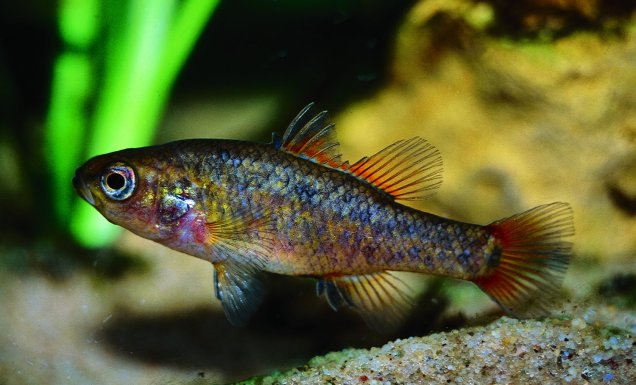
A male southern pygmy perch, which usually measures 6-8 cm long.
To my honest surprise, the paper has received a decentamount of media attention following its release. Nearly all of these have focused on the biogeographic results and interpretations of the paper, which is arguably the largest component of the paper. In these media releases, the articles are often opened with “…despite the odds, new research has shown how a tiny fish managed to find its way across the arid Australian continent – more than once.” So how did they manage it? These are tiny fish, and there’s a very large desert area right in the middle of Australia, so how did they make it all the way across? And more than once?!
The Great (southern) Southern Land
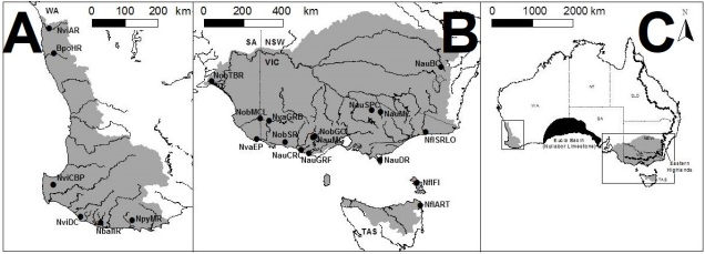
To understand the results, we first have to take a look at the context for the research question. There are seven officially named species of pygmy perches (‘named’ is an important characteristic here…but we’ll go into the details of that in another post), which are found in the temperate parts of Australia. Of these, three are found with southwest Western Australia, in Australia’s only globally recognised biodiversity hotspot, and the remaining four are found throughout eastern Australia (ranging from eastern South Australia to Tasmania and up to lower Queensland). These two regions are separated by arid desert regions, including the large expanse of the Nullarbor Plain.
The distributions of pygmy perch species across Australia. The dots and labels refer to different sampling sites used in the study. A: the distribution of western pygmy perches, and essentially the extent of the southwest WA biodiversity hotspot region. B: the distribution of eastern pygmy perches, excluding N. oxleyana which occurs in upper NSW/lower QLD (indicated in C). C: the distributions relative to the map of Australia. The black region in the middle indicates the Nullarbor Plain.
The Nullarbor Plain is a remarkable place. It’s dead flat, has no trees, and most importantly for pygmy perches, it also has no standing water or rivers. The plain was formed from a large limestone block that was pushed up from beneath the Earth approximately 15 million years ago; with the progressive aridification of the continent, this region rapidly lost any standing water drainages that would have connected the east to the west. The remains of water systems from before (dubbed ‘paleodrainages’) can be seen below the surface.
See? Nothing here. Photo taken near Watson, South Australia. Credit: Benjamin Rimmer.
Biogeography of southern Australia
As one might expect, the formation of the Nullarbor Plain was a huge barrier for many species, especially those that depend on regular accessible water for survival. In many species of both plants and animals, we see in their phylogenetic history a clear separation of eastern and western groups around this time; once widely distributed species become fragmented by the plain and diverged from one another. We would most certainly expect this to be true of pygmy perch.
But our questions focus on what happened before the Nullarbor Plain arrived in the picture. More than 15 million years ago, southern Australia was a massively different place. The climate was much colder and wetter, even in central Australia, and we even have records of tropical rainforest habitats spreading all the way down to Victoria. Water-dependent animals would have been able to cross the southern part of the continent relatively freely.
Biogeography of the enigmatic pygmy perches
This is where the real difference between everything else and pygmy perch happens. For most species, we see only one east and west split in their phylogenetic tree, associated with the Nullarbor Plain; before that, their ancestors were likely distributed across the entire southern continent and were one continuous unit.
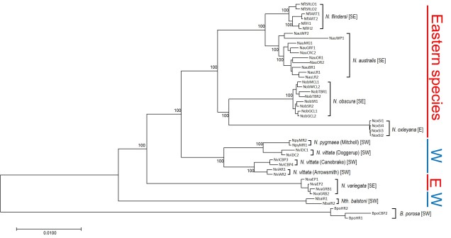
Not for pygmy perch, though. Our phylogenetic patterns show that there were multiple splits between eastern and western ancestral pygmy perch. We can see this visually within the phylogenetic tree; some western species of pygmy perches are more closely related, from an evolutionary perspective, to eastern species of pygmy perches than they are to other western species. This could imply a couple different things; either some species came about by migration from east to west (or vice versa), and that this happened at least twice, or that two different ancestral pygmy perches were distributed across all of southern Australia and each split east-west at some point in time. These two hypotheses are called “multiple invasion” and “geographic paralogy”, respectively.
The phylogeny of pygmy perches produced by this study, containing 45 different individuals across all species of pygmy perch. Species are labelled in the tree in brackets, and their geographic location (east or west) is denoted by the colour on the right. This tree clearly shows more than one E/W separation, as not all eastern species are within the same clade. For example, despite being an eastern species, N. variegata is more closely related to Nth. balstoni or N. vittata than to the other eastern species (N. australis, N. obscura, N. oxleyana and N. ‘flindersi’.
So, which is it? We delved deeper into this using a type of analysis called ‘ancestral clade reconstruction’. This tries to guess the likely distributions of species ancestors using different models and statistical analysis. Our results found that the earliest east-west split was due to the fragmentation of a widespread ancestor ~20 million years ago, and a migration event facilitated by changing waterways from the Nullarbor Plain pushing some eastern pygmy perches to the west to form the second group of western species. We argue for more than one migration across Australia since the initial ancestor of pygmy perches must have expanded from some point (either east or west) to encompass the entirety of southern Australia.
The ancestral area reconstruction of pygmy perches, estimated using the R package BioGeoBEARS. The different pie charts denote the relative probability of the possible distributions for the species or ancestor at that particular time; colours denote exactly where the distribution is (following the legend). As you can see, the oldest E/W split at 21 million years ago likely resulted from a single widespread ancestor, with it’s range split into an east and west group. The second E/W event, at 15 million years ago, most likely reflects a migration from east to west, resulting in the formation of the N. vittata species group. This coincides with the Nullarbor Plain, so it’s likely that changes in waterway patterns allowed some eastern pygmy perch to move westward as the area became more arid.
So why do we see this for pygmy perch and no other species? Well, that’s the real mystery; out of all of the aquatic species found in southeast and southwest Australia, pygmy perch are one of the worst at migrating. They’re very picky about habitat, small, and don’t often migrate far unless pushed (by, say, a flood). It is possible that unrecorded extinct species of pygmy perch might help to clarify this a little, but the chances of finding a preserved fish fossil (let alone for a fish less than 8cm in size!) is extremely unlikely. We can really only theorise about how they managed to migrate.
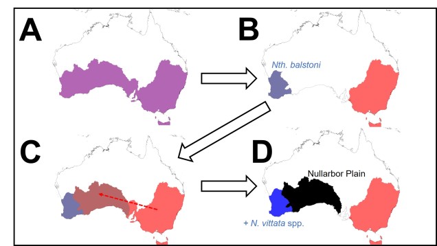
A diagram of the distribution of pygmy perch species over time, as suggested by the ancestral area reconstruction. A: the initial ancestor of pygmy perches was likely found throughout southern Australia. B: an unknown event splits the ancestor into an eastern and western group; the sole extant species of the W group is Nth. balstoni. C: the ancestor of the eastern pygmy perches spreads towards the west, entering part of the pre-Nullarbor region. D: due to changes in the hydrology of the area, some eastern pygmy perches (the maroon colour in C) are pushed towards the west; these form N. vittata species and N. pygmaea. The Nullarbor Plain forms and effectively cuts off the two groups from one another, isolating them.
What does this mean for pygmy perches?
Nearly all species of pygmy perch are threatened or worse in the conservation legislation; there have been many conservation efforts to try and save the worst-off species from extinction. Pygmy perches provide a unique insight to the history of the Australian climate and may be a key in unlocking some of the mysteries of what our land was like so long ago. Every species is important for conservation and even those small, hard-to-notice creatures that we might forget about play a role in our environmental history.
The distribution of organisms across the Earth, both over time and across space, is a fundamental aspect of the field of biogeography. But our understanding of the mechanisms by which organisms are distributed across the globe, and how this affects their evolution, can be at times highly enigmatic. Why are Australia and the Americas the only two places that have marsupials? How did lemurs get all the way to Madagascar, and why are they the only primate that has made the trip? How did Darwin’s famous finches get over to the Galápagos, and why are there so many species of them there now?
All of these questions can be addressed with a combination of genetic, environmental and ecological information across a variety of timescales. However, the overall field of biogeography (and phylogeography as a derivative of it) has traditionally been largely rooted on a strong yet changing theoretical basis. The earliest discussions and discoveries related to biogeography as a field of science date back to the 18th Century, and to Carl Linnaeus (to whom we owe our binomial classification system) and Alexander von Humboldt. These scientists (and undoubtedly many others of that era) were among the first to notice how organisms in similar climates (e.g. Australia, South Africa and South America) showed similar physical characteristics despite being so distantly separated (both in their groups and geographic distance). The communities of these regions also appeared to be highly similar. So how could this be possible over such huge distances?
A pretty unreasonable mechanism (and example) of dispersal in foxes. And yes, all tourists wear sunglasses and Hawaiian shirts, even arctic fox ones.
Dispersal or vicariance?
Two main explanations for these patterns are possible; dispersal and vicariance. As one might expect, dispersal denotes that an ancestral species was distributed in one of these places (referred to as the ‘centre of origin’) before it migrated and inhabited the other places. Contrastingly, vicariancesuggests that the ancestral species was distributed everywhere originally, covering all contemporary ranges within it. However, changes in geography, climate or the formation of other barriers caused the range of the ancestor to fragment, with each fragmented group evolving into its own distinct species (or group of species).
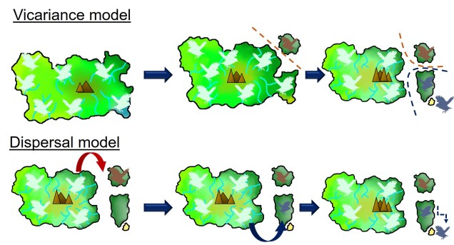
An example of dispersal vs. vicariance patterns of biogeography in an island bird (pale blue). In the top example, the sequential separation of parts of the island also cause parts of the distribution of the original bird species to become fragmented. These fragments each evolve independently of their ancestor and form new species (red, and then blue). In the bottom example, the island geography doesn’t change but in rare events a bird disperses from the main island onto a new island. The new selective pressures of that island cause the dispersed birds to evolve into new species (red and blue). In both examples, islands that were recently connected or are easy to disperse across do not generate new species (in the sandy island in the bottom right). You’ll notice that both processes result in the same biogeographic distribution of species.
In initial biogeographic science, dispersal was the most heavily favoured explanation. At the time, there was no clear mechanism by which organisms could be present all over the globe without some form of dispersal: it was generally believed that the world was a static, unmoving system. Dispersal was well supported by some biological evidence such as the diversification of Darwin’s finches across the Galápagos archipelago. Thus, this concept was supported through the proposals of a number of prominent scientists such as Charles Darwin and A.R. Wallace. For others, however, the distance required for dispersal (such as across entire oceans) seemed implausible and biologically unrealistic.
A paradigm shift in biogeography
Two particular developments in theory are credited with a paradigm shift in the field; cladistics and plate tectonics. Cladistics simply involved using shared biological characteristics to reconstruct the evolutionary relationships of species (think like phylogenetics, but using physical traits instead of genetic sequence). Just as importantly, however, was plate tectonic theory, which provided a clear way for organisms to spread across the planet. By understanding that, deep in the past, all continents had been directly connected to one another provides a convenient explanation for how species groups spread. Instead of requiring for species to travel across entire oceans, continental drift meant that one widespread and ancient ancestor on the historic supercontinent (Pangaea; or subsequently Gondwana and Laurasia) could become fragmented. It only required that groups were very old, but not necessarily very dispersive.
Surf’s up, dudes! Although continental drift was no doubt an important factor in the distribution and dispersal of many organisms on Earth, it actually probably wasn’t the reason lemurs got to Madagascar. Sorry for the mislead.
From these advances in theory, cladistic vicariance biogeography was born. The field rapidly overtook dispersal as the most likely explanation for biogeographic patterns across the globe by not only providing a clear mechanism to explain these but also an analytical framework to test questions relating to these patterns. Further developments into the analytical backbone of cladistic vicariance allowed for more nuanced questions of biogeography to be asked, although still fundamentally ignored the role of potential dispersals in explaining species’ distributions.
Modern philosophy of biogeography
So, what is the current state of the field? Well, the more we research biogeographic patterns with better data (such as with genomics) the more we realise just how complicated the history of life on Earth can be. Complex modelling (such as Bayesian methods) allow us to more explicitly test the impact of Earth history events on our study species, and can provide more detailed overview of the evolutionary history of the species (such as by directly estimating times of divergence, amount of dispersal, extent of range shifts).
From a theoretical perspective, the consistency of patterns of groups is always in question and exactly what determines what species occurs where is still somewhat debatable. However, the greater number of types of data we can now include (such as geological, paleontological, climatic, hydrological, genetic…the list goes on!) allows us to paint a better picture of life on Earth. By combining information about what we know happened on Earth, with what we know has happened to species, we can start to make links between Earth history and species history to better understand how (or if) these events have shaped evolution.