DNA – Page 6 – The G-cat

An identity crisis: using genomics to determine species identities

July 18, 2018Sean Buckley7 Comments

This is the fourth (and final) part of the miniseries on the genetics and process of speciation. To start from Part One, click here.

In last week’s post, we looked at how we can use genetic tools to understand and study the process of speciation, and particularly the transition from populations to species along the speciation continuum. Following on from that, the question of “how many species do I have?” can be further examined using genetic data. Sometimes, it’s entirely necessary to look at this question using genetics (and genomics).

Cryptic species

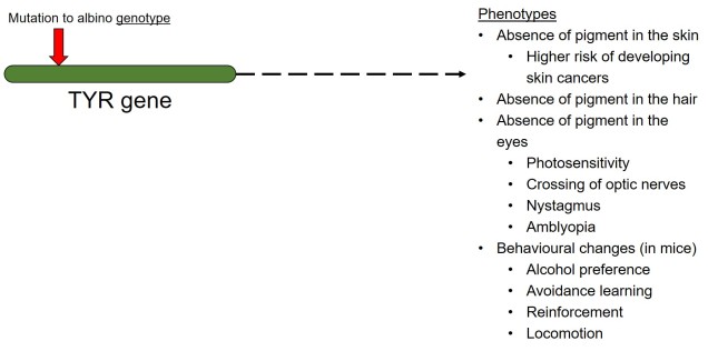
A concept that I’ve mentioned briefly previously is that of ‘cryptic species’. These are species which are identifiable by their large genetic differences, but appear the same based on morphological, behavioural or ecological characteristics. Cryptic species often arise when a single species has become fragmented into several different populations which have been isolated for a long time from another. Although they may diverge genetically, this doesn’t necessarily always translate to changes in their morphology, ecology or behaviour, particularly if these are strongly selected for under similar environmental conditions. Thus, we need to use genetic methods to be able to detect and understand these species, as well as later classify and describe them.

Cryptic species heatmap example — The level of genetic differentiation between the fish in the above example. The phylogenies on the left and top of the figure demonstrate the evolutionary relationships of these four fish. The matrix shows a heatmap of the level of differences between different pairwise comparisons of all four fish: red squares indicate zero genetic differences (such as when comparing a fish to itself; the middle diagonal) whilst yellow squares indicate increasingly higher levels of genetic differentiation (with bright yellow = all differences). By comparing the different fish together, we can see that Fish 1 and 2, and Fish 3 and 4, are relatively genetically similar to one another (red-deep orange). However, other comparisons show high level of genetic differences (e.g. 1 vs 3 and 1 vs 4). Based on this information, we might suggest that Fish 1 and 2 belong to one cryptic species (A) and Fish 3 and 4 belong to a second cryptic species (B).

Genetic tools to study species: the ‘Barcode of Life’

A classically employed method that uses DNA to detect and determine species is referred to as the ‘Barcode of Life’. This uses a very specific fragment of DNA from the mitochondria of the cell: the cytochrome c oxidase I gene, CO1. This gene is made of 648 base pairs and is found pretty well universally: this and the fact that CO1 evolves very slowly make it an ideal candidate for easily testing the identity of new species. Additionally, mitochondrial DNA tends to be a bit more resilient than its nuclear counterpart; thus, small or degraded tissue samples can still be sequenced for CO1, making it amenable to wildlife forensics cases. Generally, two sequences will be considered as belonging to different species if they are certain percentage different from one another.

Annotated mitogeome — The full (annotated) mitochondrial genome of humans, with the different genes within it labelled. The CO1 gene is labelled with the red arrow (sometimes also referred to as COX1) whilst blue arrows point to other genes often used in phylogenetic or taxonomic studies, depending on the group or species in question.

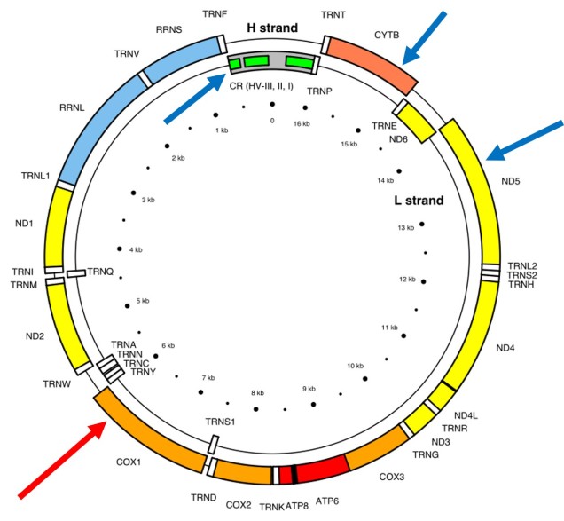
Despite the apparent benefits of CO1, there are of course a few drawbacks. Most of these revolve around the mitochondrial genome itself. Because mitochondria are passed on from mother to offspring (and not at all from the father), it reflects the genetic history of only one sex of the species. Secondly, the actual cut-off for species using CO1 barcoding is highly contentious and possibly not as universal as previously suggested. Levels of sequence divergence of CO1 between species that have been previously determined to be separate (through other means) have varied from anywhere between 2% to 12%. The actual translation of CO1 sequence divergence and species identity is not all that clear.

Gene tree – species tree incongruences

One particularly confounding aspect of defining species based on a single gene, and with using phylogenetic-based methods, is that the history of that gene might not actually be reflective of the history of the species. This can be a little confusing to think about but essentially leads to what we call “gene tree – species tree incongruence”. Different evolutionary events cause different effects on the underlying genetic diversity of a species (or group of species): while these may be predictable from the genetic sequence, different parts of the genome might not be as equally affected by the same exact process.

A classic example of this is hybridisation. If we have two initial species, which then hybridise with one another, we expect our resultant hybrids to be approximately made of 50% Species A DNA and 50% Species B DNA (if this is the first generation of hybrids formed; it gets a little more complicated further down the track). This means that, within the DNA sequence of the hybrid, 50% of it will reflect the history of Species A and the other 50% will reflect the history of Species B, which could differ dramatically. If we randomly sample a single gene in the hybrid, we will have no idea if that gene belongs to the genealogy of Species A or Species B, and thus we might make incorrect inferences about the history of the hybrid species.

Gene tree incongruence figure — A diagram of gene tree – species tree incongruence. Each individual coloured line represents a single gene as we trace it back through time; these are mostly bound within the limits of species divergences (the black borders). For many genes (such as the **blue** ones), the genes resemble the pattern of species divergences very well, albeit with some minor differences in how long ago the splits happened (at the top of the branches). However, the **red** genes contrast with this pattern, with clear movement across species (from A and C into B): this represents genes that have been transferred by hybridisation. The **green** line represents a gene affected by what we call incomplete lineage sorting; that is, we cannot trace it back far enough to determine exactly how/when it initially diverged and so there are still two separate green lines at the very top of the figure. You can think of each line as a separate phylogenetic tree, with the overarching species tree as the **average pattern** of all of the genes.

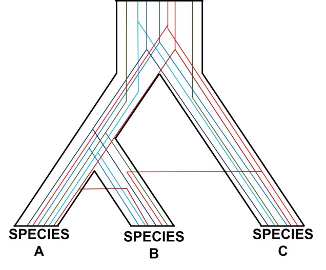
There are a number of other processes that could similarly alter our interpretations of evolutionary history based on analysing the genetic make-up of the species. The best way to handle this is simply to sample more genes: this way, the effect of variation of evolutionary history in individual genes is likely to be overpowered by the average over the entire gene pool. We interpret this as a set of individual gene trees contained within a species tree: although one gene might vary from another, the overall picture is clearer when considering all genes together.

Species delimitation

In earlier posts on The G-CAT, I’ve discussed the biogeographical patterns unveiled by my Honours research. Another key component of that paper involved using statistical modelling to determine whether cryptic species were present within the pygmy perches. I didn’t exactly elaborate on that in that section (mostly for simplicity), but this type of analysis is referred to as ‘species delimitation’. To try and simplify complicated analyses, species delimitation methods evaluate possible numbers and combinations of species within a particular dataset and provides a statistical value for which configuration of species is most supported. One program that employs species delimitation is Bayesian Phylogenetics and Phylogeography (BPP): to do this, it uses a plethora of information from the genetics of the individuals within the dataset. These include how long ago the different populations/species separated; which populations/species are most related to one another; and a pre-set minimum number of species (BPP will try to combine these in estimations, but not split them due to computational restraints). This all sounds very complex (and to a degree it is), but this allows the program to give you a statistical value for what is a species and what isn’t based on the genetics and statistical modelling.

Vittata cryptic species — The cryptic species of pygmy perches identified within my research paper. This represents part of the main phylogenetic tree result, with the estimates of divergence times from other analyses included. The pictures indicate the physiology of the different ‘species’: Nannoperca pygmaea is morphologically different to the other species of Nannoperca vittata. Species delimitation analysis suggested all four of these were genetically independent species; at the very least, it is clear that there must be at least 2 species of Nannoperca vittata since A is more related to N. pygmaea than to other N. vittata species. Photo credits: N. vittata = Chris Lamin; N. pygmaea = David Morgan.

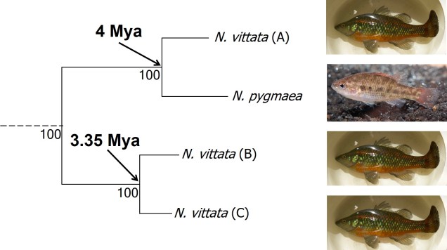
The end result of a BPP run is usually reported as a species tree (e.g. a phylogenetic tree describing species relationships) and statistical support for the delimitation of species (0-1 for each species). Because of the way the statistical component of BPP works, it has been found to give extremely high support for species identities. This has been criticised as BPP can, at time, provide high statistical support for genetically isolated lineages (i.e. divergent populations) which are not actually species.

Improving species identities with integrative taxonomy

Due to this particular drawback, and the often complex nature of species identity, using solely genetic information such as species delimitation to define species is extremely rare. Instead, we use a combination of different analytical techniques which can include genetic-based evaluations to more robustly assign and describe species. In my own paper example, we suggested that up to three ‘species’ of N. vittata that were determined as cryptic species by BPP could potentially exist pending on further analyses. We did not describe or name any of the species, as this would require a deeper delve into the exact nature and identity of these species.

As genetic data and analytical techniques improve into the future, it seems likely that our ability to detect and determine species boundaries will also improve. However, the additional supported provided by alternative aspects such as ecology, behaviour and morphology will undoubtedly be useful in the progress of taxonomy.

The direction of evolution: divergence vs. convergence

June 6, 2018June 7, 2018Sean Buckley6 Comments

Direction of evolution

We’ve talked previously on The G-CAT about how the genetic underpinning of certain evolutionary traits can change in different directions depending on the selective pressure it is under. Particularly, we can see how the frequency of different alleles might change in one direction or another, or stabilise somewhere in the middle, depending on its encoded trait. But thinking bigger picture than just the genetics of one trait, we can actually see that evolution as an entire process works rather similarly.

Divergent evolution

The classic view of the direction of evolution is based on divergent evolution. This is simply the idea that a particular species possess some ancestral trait. The species (or population) then splits into two (for one reason or another), and each one of these resultant species and populations evolves in a different way to the other. Over time, this means that their traits are changing in different directions, but ultimately originate from the same ancestral source.

Evidence for divergent evolution is rife throughout nature, and is a fundamental component of all of our understanding of evolution. Divergent evolution means that, by comparing similar traits in two species (called homologous traits), we can trace back species histories to common ancestors. Some impressive examples of this exist in nature, such as the number of bones in most mammalian species. Humans have the same number of neck bones as giraffes; thus, we can suggest that the ancestor of both species (and all mammals) probably had a similar number of neck bones. It’s just that the giraffe lineage evolved longer bones whereas other lineages did not.

Homology figure — A diagrammatic example of homologous structures in ‘hand’ bones. The coloured bones demonstrate how the same original bone structures have diverged into different forms. Source: BiologyWise.

Convergent evolution

But of course, evolution never works as simply as you want it to, and sometimes we can get the direct opposite pattern. This is called convergent evolution, and occurs when two completely different species independently evolve very similar (sometimes practically identical) traits. This is often caused by a limitation of the environment; some extreme demand of the environment requires a particular physiological solution, and thus all species must develop that trait in order to survive. An example of this would be the physiology of carnivorous marsupials like Tasmanian devils or thylacines: despite being in another Class, their body shapes closely resemble something more canid. Likely, the carnivorous diet places some constraints on physiology, particularly jaw structure and strength.

Convergent evol intelligence — A surprising example of convergent evolution is cognitive ability in apes and some bird groups (e.g. corvids). There’s plenty of other animal groups more related to each of these that don’t demonstrate the same level of cognitive reasoning (based on the traits listed in the centre): thus, we can conclude that cognition has evolved twice in very, very different lineages. Source: Emery & Clayton, 2004.

A more dramatic (and potentially obvious) example of convergent evolution would be wings and the power of flight. Despite the fact that butterflies, bees, birds and bats all have wings and can fly, most of them are pretty unrelated to one another. It seems much more likely that flight evolved independently multiple times, rather than the other 99% of species that shared the same ancestor lost the capacity of flight.

Parallel evolution

Sometimes convergent evolution can work between two species that are pretty closely related, but still evolved independently of one another. This is distinguished from other categories of evolution as parallel evolution: the main difference is that while both species may have shared the same start and end point, evolution has acted on each one independent of the other. This can make it very difficult to diagnose from convergent evolution, and is usually determined by the exact history of the trait in question.

Parallel evolution is an interesting field of research for a few reasons. Firstly, it provides a scenario in which we can more rigorously test expectations and outcomes of evolution in a particular environment. For example, if we find traits that are parallel in a whole bunch of fish species in a particular region, we can start to look at how that particular environment drives evolution across all fish species, as opposed to one species case studies.

Marsupial handedness.jpg — Here’s another weird example; different populations of marsupials (particularly kangaroos and wallabies) show preferential handedness depending on where the population is. That is, different populations of different species of marsupials shows parallel evolution of handedness, since they’re related to one another but have evolved it independently of the other species. Source: Giljov et al. (2015).

Following from that logic, it is then important to question the mechanisms of parallelism. From a genetic point of view, do these various species use the same genes (and genetic variants) to produce the same identical trait? Or are there many solutions to the selective question in nature? While these questions are rather complicated, and there has been plenty of evidence both for and against parallel genetic underpinning of parallel traits, it seems surprisingly often that many different genetic combinations can be used to get the same result. This gives interesting insight into how complex genetic coding of traits can be, and how creative and diverse evolution can be in the real world.

Where is evolution going?

Cat phylogeny — An example of all three types of evolutionary trajectory in a single phylogeny of cats (you know how we do it here at The G-CAT). This phylogeny consists of two distinct genera; one with one species (P. aliquam) and another of three species (the red box indicates their distance). Our species have three main physical traits: coat colour, ear tufts and tail shape. At the ancestral nodes of the tree, we can see what the ancestor of these species looked like for these three traits. Each of these traits has undergone a different type of evolution. The tufts on the ears are the result of divergent evolution, since F. tuftus evolved the trait differently to its nearest relative, F. griseo. Contrastingly, the orange coat colour of F. tuftus and P. aliquam are the result of convergent evolution: neither of these species are very closely related (remembering the red box) and evolved orange coats independently of one another (since their ancestors are grey). And finally, the fluffy tails of F. hispida and F. griseo can be considered parallel evolution, since they’re similar evolutionarily (same genus) but still each evolved tail fluff independently (not in the ancestor). This example is a little convoluted, but if you trace the history of each trait in the phylogeny you can more easily see these different patterns.

So, where is evolution going for nature? Well, the answer is probably all over the place, but steered by the current environmental circumstances. Predicting the evolutionary impacts of particular environmental change (e.g. climate change) is exceedingly difficult but a critical component of understanding the process of evolution and the future of species. Evolution continually surprises us with creative solution to complex problems and I have no doubt new mysteries will continue to be thrown at us as we delve deeper.

All the world in the palm of your hand: whole genome sequencing for evolution and conservation

May 30, 2018Sean Buckley4 Comments

Building an entire genome

If bigger is better, then biggest is best. Having the genome of a particular study species fully sequenced allows us to potentially look at all of the genetic variation in the entire gene pool: but how do we sequence the entirety of the genome? And what are the benefits of having a whole genome to refer to?

Whole genome assembly — A very, very simplified overview of whole genome sequencing. Similar to other genomic technologies, we start by fragmenting the genome into much smaller, easier to sequence parts (reads). We then use a computer algorithm which pieces these reads together into a consecutive sequence based on overlapping DNA sequence (like building a chain out of Lego blocks). From this assembled genome, we can then attach annotations using information from other species’ genomes or genetic studies, which can correlate a particular sequence to a gene, a function of that gene, and the resultant protein from these gene (although not always are all of these aspects included).

Well, assembling the whole genome of an organism for the first time is a very tricky process. It involves taking DNA sequence from only a few individuals, breaking them down into smaller fragments and multiplying these fragments into the billions (moreorless the same process used in other genomics technologies: the real difference is that we need the full breadth of the genome so that we don’t miss any spaces). From these fragments, we use a complex computer algorithm which builds up a consensus sequence like a Lego tower; by finding parts of sequences which overlap, the software figures out which pieces connect to one another. Hopefully, we eventually end up with one very long continuous sequence; the genome! Sometimes, we might end with a few very large blocks (called contigs), but this is also useful for analyses (correlated with how many/big blocks there are). With this full genome, we use information from other more completed genomes (such as those from model species like humans, mice or even worms) to figure out which sections of the genome relate to specific genes. We can then annotate these sections by labelling them as clear genes, complete with start and end point, and attach a particular physical function of that gene.

The benefits of whole genomes

Having an entire genome as a reference is an extremely helpful tool in conservation and evolutionary studies. The first, and perhaps most obvious benefit, is the sheer scale of the data we can use. By having the entirety of the genome available, we can use potentially billions of base pairs of sequence in our genetic analyses (for reference, the human genome is >3 billion base pairs long). Even if we don’t sequence the full genome for all of our samples, having a reference genome as basis for assembly our reduced datasets significantly improves the quantity and quality of sequences we can use.

Another very important benefit is the ability to prescribe function in our studies. Many of our processes for obtaining data, even for genomic technologies, use random and anonymous fragments of the genome. Although this is a cost-effective way to obtain a very large amount of data, it unfortunately means that we often have no idea which part of the genome our sequences came from. This means that we don’t know which sequences relate to specific genes, and even if we did we would have no idea what those genes are or do! But with an annotated genome, we can take even our fragmented sequence and check it against the genome and find out what genes are present.

Understanding adaptation

Based on that, it seems pretty obvious about exactly how having an annotated genome can help us in studies of adaptation. Knowing the functional aspect of our genetic data allows us to more directly determine how evolution is happening in nature; instead of only being able to say that two species are evolving differently from one another, for example, we can explicitly look at how they are evolving. Is one evolving tolerance to hotter temperatures? Are they evolving different genes to handle different diets? Are they evolving in response to an external influence, like a viral outbreak or changing climate? What are the physiological consequences of these changes? These questions are critical in understanding past and future evolution, and full genome analysis allows us to delve into them much deeper.

Manhattan plot example — A (slightly edited) figure of full genome comparisons between domestic dogs and wild wolves by Axelsson *et al.* (2013), with the aim of understanding the evolutionary changes associated with domestication. For avid readers, this figure probably looks familiar. This figure compares the genetic differentiation across the entire genome between dogs and wolves, with some sections of the genome (circled) showing clear differences. As there is an annotated dog genome, the authors then delved into these genes to understand the functional differences between the two. By comparing their genetic differences to functional genes, the authors can more explicitly suggest mechanisms or changes associated with the domestication process (such as adaptation to a starch-heavy and human-influenced diet).

This includes allowing us to better understand how adaptation actually works in nature. As we’ve discussed before, more traditional studies often assumed that single, or very few, genes were responsible for allowing a species to adapt and change, and that these genes had very strong effects on their physiology. But what we see far more often is polygenic adaptation; small changes in a very large number of genes which, combined together, allow the species to adapt and evolve. By having the entirety of the genome available, we are much more likely to capture all of the genes that are under natural selection in a particular population or species, painting a clearer picture of their evolutionary trajectory.

Understanding demography

The much larger dataset of full genomes is also important for understanding the non-adaptive parts of evolution; the demographic history. Given that selectively neutral impacts (e.g. reductions in population size) are likely to impact all of the genes in the gene pool somewhat equally, having a full genome allows us to more accurately infer the demographic state and historical patterns of species.

For both adaptive and non-adaptive variation, it is also important to consider what we call linkage disequilibrium. Genetic sequences that are physically close to each other in the genome will often be inherited together due to the imprecision of recombination (a fairly technical process, so I won’t delve into this): what this can mean is that if a gene is under very strong selection, then sequences around this gene will also look like they’re under selection too. This can give falsely positive adaptive genes (i.e. sequences that look like genes under selection but are just linked to a gene that is) or can interfere with demographic analyses (since they often assume no selection, or linkage to selection, on the sequences used). With a whole genome, we can actually estimate how far away a base pair has to be before it’s not linked anymore; we call these linkage blocks, and they’re very useful additions to analyses.

Linkage_example — An example of linkage as a process. We start with a particular sequence (top); during recombination, this sequence may randomly break and rearrange into different parts. In this example, I’ve simulated four different ‘breaks’ (dashed coloured lines) due to recombination. Each of these breaks leads to two separate blocks of fragments; for example, the break at the blue line results in the second two sequence blocks (middle). If we focus on one target base pair in the sequence (golden A), then we can see in some fragments it remains with certain bases, but sometimes it gets separated by the break. If we compare how often the golden A is in the same block (i.e. is co-inherited) as each of the other bases, across all 4 breaks, then we see that the bases that are closest to it (the golden A is represented by the golden bar) are almost always in the same block. This makes sense: the further away a base is from our target, the more likely that there will be a break between it. This is shown in the frequency distributions at the bottom: the left figure shows the actual frequencies of co-inheritance (i.e. linkage) using the top example and those 4 breaks. The right figure shows a more realistic depiction of how linkage looks in the genome; it rapidly decays as we move away from the target (although the width and rate of this can vary).

Improving conservation management

In a similar fashion to demography, full genome datasets can improve our estimates of relatedness and pedigrees in captive breeding programs. The massive scale of whole genomes allows us to more easily trace the genealogical history of individuals, allowing us to assign parents more accurately. This also helps with our estimations of genetic relatedness, arguably the most critical aspect of genetic-based breeding programs. This is particularly helpful for species with tricky mating patterns, such as polyamory, brood spawning or difficult to track organisms.

The way forwards

While many non-model species are still lacking in the available genomic information, whole genomes are progressively being sequenced for more and more species. As this astronomical dataset grows, our ability to investigate, discover and test theories about evolution, natural selection and conservation will also improve. Many projects already exist which aim specifically to increase the number of whole genomes available for certain taxonomic groups such as birds and bats: these will no doubt prove to be invaluable resources for future studies.

Why we should always pander to diversity

May 16, 2018Sean Buckley5 Comments

Diversity in the natural world

‘Diversity’ is a term that gets used a lot these days, albeit usually in reference to social changes and structures. However, diversity is not merely a human construct and reflects an extremely important aspect of the natural world at a variety of levels. From the smallest genes to the biggest ecosystems, diversity is a trait that confers a massive range of benefits to individuals, populations, species and even the entire globe. Let’s dissect this diversity down at different scales and see how beneficial it can be.

Hierarchy of diversity — The generalised hierarchy at life, with diversity being an important component of each tier. At the smallest tier, genes underpin all life. The collection of genetic diversity is often summarised into a population (as a single cohesive genetic unit). Several populations can be pooled together into a single (usually) cohesive species. Different species are then components of a larger community (which in turn are components of a broader ecosystem).

Genetic diversity

At the smallest scale in the hierarchy of genetic differentiation, we have the genes themselves. It is a well-established concept that having a diversity of genetic variants (alleles) within a population or species is critical to their future adaptation, evolution and persistance. This is because different alleles will have different benefits (or costs) depending on the environmental pressure that influences them; natural selection might favour one allele over another at one time, but a different one as the pressure changes. Having a higher number of alleles within the population or species means that there is a greater chance at least a few individuals will possess an adaptive gene with the changing environment (which we know can be quite rapid and very, very strong). The diversity serves as a ‘buffer’ against extinction; evolution by natural selection functions best when there are many options to choose from.

Without this diversity, species run the risk of having no adaptive genes at the ready to deal with a selective pressure. Either a new adaptive gene must mutate (or come about in other ways, such as through gene flow from another population or species) or the population/species will suffer and potentially go extinct. As strong selection causes the species to dwindle, it enters what is referred to as the ‘extinction vortex’. Without genetic diversity, they can’t adapt: thus, more individuals die off, causing more genetic diversity to be lost from the population. This pattern is a vicious cycle which can inevitably destroy species (without serious intervention).

Extinction vortex — A very dramatic representation of the extinction vortex.

For this reason, captive breeding programs aim to maintain as much of the genetic diversity of the original population as possible. This reduces the probability of entering a downward extinction spiral from inbreeding depression and helps to maintain populations into the future (both the captive one and the wild population when we reintroduce individuals into the wild).

“Population” diversity

Because genetic diversity is critically important for species survival, we must also try to preserve the diversity of the entire gene pool of a species. This means conserving highly genetically differentiated populations within a species as a priority, as they may be the only ones that possess the necessary adaptive genes to save the rest of the species. This adaptive genetic variation can then be introduced into other populations in genetic rescue programs and serve as a means to semi-naturally allow the species to evolve. Evolutionarily-significant units (ESUs) are one measure of the invaluable nature of genetically unique populations.

Although many more traditional conservationists strongly believe that ESUs should be managed entirely independently of one another (to preserve their evolutionary ‘pedigree’ and prevent the risk of outbreeding depression), it has been suggested that the benefit of genetic rescue in many cases significantly outweighs this risk of outbreeding depression. For some species, this really is an act of rescue: they are at the edge of extinction, and if we do nothing we condemn them to die out.

Introducing genetic material across populations (or even species!) can generate new functional genes that allow the recipient species to adapt to selective pressures. This might sound very strange, and could be extremely rare, but examples of adaptive genetic material in one species originating from another species through hybridisation do exist in nature. For example, the black coat of wolves is a highly adaptive trait in some populations and is encoded for by the Melanocortin 1 receptor (Mc1r) gene. However, the specific mutation in Mc1r gene that generates the black coat colour actually first originated in domestic dogs; when wild wolves and domestic dogs interbred, this mutation was transferred into the wolf gene pool. Natural selection strongly favoured this new variant, and it very rapidly underwent strong positive selection. Thus, the adaptiveness of black wolves is thanks to a domestic dog mutation!

Species diversity

At a higher level of the hierarchy, the diversity of species within a particular community or ecosystem has been shown to be important for the health and stability of said community. Every species, however small or seemingly unimpressive, plays a role in the greater ecosystem balance, through interactions with other species (e.g. as predator, as prey, as competitor) and the abiotic environment. While some species are known to have very strong impacts on the immediate ecosystem (often dubbed ‘keystone species’, such as apex predators), all species have some influence on the world around them (we’re especially good at it).

Species interactions flowchart

The overall health and stability of an ecosystem, as well as the benefits it can provide to all living things (including humans) is largely determined by the diversity of species. For example, ‘habitat engineers’ are types of species that, by altering the physical environment around them (such as to build a home), directly provide new habitat for other species. They are a fundamental underpinning of many incredibly vibrant ecosystems; think of what a reef system would look like if there were no corals in it. There’d be no anemones growing colourfully; no fish to live in them; no sharks to feed on these non-existent fish. This is just one example of a complex ecosystem that truly relies on its inhabiting species to function.

Ecosystem jenga — Much like Jenga, taking out one block (a species) could cause the entire stack (the ecosystem) to collapse in on itself. Even if it stands up, however, the system will still be weaker without the full diversity to support it.

Protecting our diversity

Diversity is not just a social construct and is an important phenomenon in nature, at a variety of different levels. Preserving the full diversity of life, from genetic diversity within populations and species to full species diversity within ecosystems, is critical to maintaining healthy and robust natural systems. The more diversity we have at each level of this hierarchy, the greater robustness and security we will have in the future.

The many genetic faces of adaptation

April 5, 2018April 6, 2018Sean Buckley15 Comments

The transition from genotype to phenotype

While evolutionary genetics studies often focus on the underlying genetic architecture of species and populations to understand their evolution, we know that natural selection acts directly on physical characteristics. We call these the phenotype; by studying changes in the genes that determine these traits (the genotype), we can take a nuanced approach at studying adaptation. However, our ability to look at genetic changes and relate these to a clear phenotypic trait, and how and why that trait is under natural selection, can be a difficult task.

One gene for one trait

The simplest (and most widely used) models of understanding the genetic basis of adaptation assume that a single genotype codes for a single phenotypic trait. This means that changes in a single gene (such as outliers that we have identified in our analyses) create changes in a particular physical trait that is under a selective pressure in the environment. This is a useful model because it is statistically tractable to be able to identify few specific genes of very large effect within our genomic datasets and directly relate these to a trait: adding more complexity exponentially increases the difficulty in detecting patterns (at both the genotypic and phenotypic level).

Single locus figure — An example of a single gene coding for a single phenotypic trait. In this example, the different combination of alleles of the one gene determines the colour of the cat.

Many genes for one trait: polygenic adaptation

Unfortunately, nature is not always convenient and recent findings suggest that the overwhelming majority of the genetics of adaptation operate under what is called ‘polygenic adaptation’. As the name suggestions, under this scenario changes (even very small ones) in many different genes combine together to have a large effect on a particular phenotypic trait. Given the often very small magnitude of the genetic changes, it can be extremely difficult to separate adaptive changes in genes from neutral changes due to genetic drift. Likewise, trying to understand how these different genes all combine into a single functional trait is almost impossible, especially for non-model species.

Polygenic adaptation is often seen for traits which are clearly heritable, but don’t show a single underlying gene responsible. Previously, we’ve covered this with the heritability of height: this is one of many examples of ‘quantitative trait loci’ (QTLs). Changes in one QTL (a single gene) causes a small quantitative change in a particular trait; the combined effect of different QTLs together can ‘add up’ (or counteract one another) to result in the final phenotype value.

Height QTL — An example of polygenic quantitative trait loci. In this example, height is partially coded for by a total of ten different genes: the dominant form of each gene (Capitals, green) provides more height whereas the recessive form (lowercase, red) doesn’t. The cumulative total of these components determines how tall the person is: the person on the far right was very unlucky and got 0/10 height bonuses and so is the shortest. Progressively from left to right, some genes are contributing to the taller height of the people, with the far right person standing tall with the ultimate 10/10 pro-height genes. For reference, height is actually likely to be coded for by thousands of genes, not 10.

The mechanisms which underlie polygenic adaptation can be more complex than simple addition, too. Individual genes might cause phenotypic changes which interact with other phenotypes (and their underlying genotypes) to create a network of changes. We call these interactions ‘epistasis’, where changes in one gene can cause a flow-on effect of changes in other genes based on how their resultant phenotypes interact. We can see this in metabolic pathways: given that a series of proteins are often used in succession within pathways, a change in any single protein in the process could affect every other protein in the pathway. Of course, knowing the exact proteins coded for every gene, including their physical structure, and how each of those proteins could interact with other proteins is an immense task. Similar to QTLs, this is usually limited to model species which have a large history of research on these specific areas to back up the study. However, some molecular ecology studies are starting to dive into this area by identifying pathways that are under selection instead of individual genes, to give a broader picture of the overall traits that are underlying adaptation.

Labrador epistasis figure — My favourite example of epistasis on coat colour in labradors. Two genes together determine the colour of the coat, with strong interactions between them. The first gene (E/e) determines whether or not the underlying coat gene (B/b) is masked or not: two recessive alleles of the first gene (ee) completely blocks Gene 2 and causes the coat to become golden regardless of the second gene genotype (much like my beloved late childhood pet pictured, Sunny). If the first gene has at least one dominant allele, then the second gene is allowed to express itself. Possessing a dominant allele (BB or Bb) leads to a black lab; possessing two recessive alleles (bb) makes a choc lab!

Labrador epistasis table — The possible combinations of genotypes for the two above genes and the resultant coat colour (indicated by the box colour).

One gene for many traits: pleiotropy and differential gene expression

In contrast to polygenic traits, changes in a single gene can also potentially alter multiple phenotypic traits simultaneously. This is referred to as ‘pleiotropy’ and can happen if a gene has multiple different functions within an organism; one particular protein might be a component of several different systems depending on where it is found or how it is arranged. A clear example of pleiotropy is in albino animals: the most common form of albinism is the result of possessing two recessive alleles of a single gene (TYR). The result of this is the absence of the enzyme tyrosinase in the organism, a critical component in the production of melanin. The flow-on phenotypic effects from the recessive gene most obviously cause a lack of pigmentation of the skin (whitening) and eyes (which appear pink), but also other physiological changes such as light sensitivity or total blindness (due to changes in the iris). Albinism has even been attributed to behavioural changes in wild field mice.

Albinism pleiotropy — A very simplified diagram of how one genotype (the albino version of the TYR gene) can lead to a large number of phenotypic changes via pleiotropy (although many are naturally physiologically connected).

Because pleiotropic genes code for several different phenotypic traits, natural selection can be a little more complicated. If some resultant traits are selected against, but others are selected for, it can be difficult for evolution to ‘resolve’ the balance between the two. The overall fitness of the gene is thus dependent on the balance of positive and negative fitness of the different traits, which will determine whether the gene is positively or negatively selected (much like a cost-benefit scenario). Alternatively, some traits which are selectively neutral (i.e. don’t directly provide fitness benefits) may be indirectly selected for if another phenotype of the same underlying gene is selected for.

Multiple phenotypes from a single ‘gene’ can also arise by alternate splicing: when a gene is transcribed from the DNA sequence into the protein, the non-coding intron sections within the gene are removed. However, exactly which introns are removed and how the different coding exons are arranged in the final protein sequence can give rise to multiple different protein structures, each with potentially different functions. Thus, a single overarching gene can lead to many different functional proteins. The role of alternate splicing in adaptation and evolution is a rarely explored area of research and its importance is relatively unknown.

Non-genes for traits: epigenetics

This gets more complicated if we consider ‘non-genetic’ aspects underlying the phenotype in what we call ‘epigenetics’. The phrase literally translates as ‘on top of genes’ and refers to chemical attachments to the DNA which control the expression of genes by allowing or resisting the transcription process. Epigenetics is a relatively new area of research, although studies have started to delve into the role of epigenetic changes in facilitating adaptation and evolution. Although epigenetics is still a relatively new research topic, future research into the relationship between epigenetic changes and adaptive potential might provide more detailed insight into how adaptation occurs in the wild (and might provide a mechanism for adaptation for species with low genetic diversity)!

The different interactions between genotypes, phenotypes and fitness, as well as their complex potential outcomes, inevitably complicates any study of evolution. However, these are important aspects of the adaptation process and to discard them as irrelevant will not doubt reduce our ability to examine and determine evolutionary processes in the wild.