Bringing alleles back together: applications of coalescent theory

Coalescent theory

A recurring analytical method, both within The G-CAT and the broader ecological genetic literature, is based on coalescent theory. This is based on the mathematical notion that mutations within genes (leading to new alleles) can be traced backwards in time, to the point where the mutation initially occurred. Given that this is a retrospective, instead of describing these mutation moments as ‘divergence’ events (as would be typical for phylogenetics), these appear as moments where mutations come back together i.e. coalesce.

There are a number of applications of coalescent theory, and it is particularly fitting process for understanding the demographic (neutral) history of populations and species.

Mathematics of the coalescent

Before we can explore the multitude of applications of the coalescent, we need to understand the fundamental underlying model. The initial coalescent model was described in the 1980s, built upon by a number of different ecologists, geneticists and mathematicians. However, John Kingman is often attributed with the formation of the original coalescent model, and the Kingman’s coalescent is considered the most basic, primal form of the coalescent model.

From a mathematical perspective, the coalescent model is actually (relatively) simple. If we sampled a single gene from two different individuals (for simplicity’s sake, we’ll say they are haploid and only have one copy per gene), we can statistically measure the probability of these alleles merging back in time (coalescing) at any given generation. This is the same probability that the two samples share an ancestor (think of a much, much shorter version of sharing an evolutionary ancestor with a chimpanzee).

Normally, if we were trying to pick the parents of our two samples, the number of potential parents would be the size of the ancestral population (since any individual in the previous generation has equal probability of being their parent). But from a genetic perspective, this is based on the genetic (effective) population size (Ne), multiplied by 2 as each individual carries two copies per gene (one paternal and one maternal). Therefore, the number of potential parents is 2Ne.

Constant Ne and coalescent prob
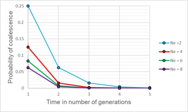
A graph of the probability of a coalescent event (i.e. two alleles sharing an ancestor) in the immediately preceding generation (i.e. parents) relatively to the size of the population. As one might expect, with larger population sizes there is low chance of sharing an ancestor in the immediately prior generation, as the pool of ‘potential parents’ increases.

If we have an idealistic population, with large Ne, random mating and no natural selection on our alleles, the probability that their ancestor is in this immediate generation prior (i.e. share a parent) is 1/(2Ne). Inversely, the probability they don’t share a parent is 1 − 1/(2Ne). If we add a temporal component (i.e. number of generations), we can expand this to include the probability of how many generations it would take for our alleles to coalesce as (1 – (1/2Ne))t-1 x 1/2Ne.
Variable Ne and coalescent probs
The probability of two alleles sharing a coalescent event back in time under different population sizes. Similar to above, there is a higher probability of an earlier coalescent event in smaller populations as the reduced number of ancestors means that alleles are more likely to ‘share’ an ancestor. However, over time this pattern consistently decreases under all population size scenarios.

Although this might seem mathematically complicated, the coalescent model provides us with a scenario of how we would expect different mutations to coalesce back in time if those idealistic scenarios are true. However, biology is rarely convenient and it’s unlikely that our study populations follow these patterns perfectly. By studying how our empirical data varies from the expectations, however, allows us to infer some interesting things about the history of populations and species.

Testing changes in Ne and bottlenecks

One of the more common applications of the coalescent is in determining historical changes in the effective population size of species, particularly in trying to detect genetic bottleneck events. This is based on the idea that alleles are likely to coalesce at different rates under scenarios of genetic bottlenecks, as the reduced number of individuals (and also genetic diversity) associated with bottlenecks changes the frequency of alleles and coalescence rates.

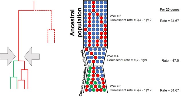
For a set of k different alleles, the rate of coalescence is determined as k(k – 1)/4Ne. Thus, the coalescence rate is intrinsically linked to the number of genetic variants available: Ne. During genetic bottlenecks, the severely reduced Ne gives the appearance of coalescence rate speeding up. This is because alleles which are culled during the bottleneck event by genetic drift causes only a few (usually common) alleles to make it through the bottleneck, with the mutation and spread of these alleles after the bottleneck. This can be a little hard to think of, so the diagram below demonstrates how this appears.
Bottleneck test figure.jpg
A diagram of how the coalescent can be used to detect bottlenecks in a single population (centre). In this example, we have contemporary population in which we are tracing the coalescence of two main alleles (red and green, respectively). Each circle represents a single individual (we are assuming only one allele per individual for simplicity, but for most animals there are up to two).  Looking forward in time, you’ll notice that some red alleles go extinct just before the bottleneck: they are lost during the reduction in Ne. Because of this, if we measure the rate of coalescence (right), it is much higher during the bottleneck than before or after it. Another way this could be visualised is to generate gene trees for the alleles (left): populations that underwent a bottleneck will typically have many shorter branches and a long root, as many branches will be ‘lost’ by extinction (the dashed lines, which are not normally seen in a tree).

This makes sense from theoretical perspective as well, since strong genetic bottlenecks means that most alleles are lost. Thus, the alleles that we do have are much more likely to coalesce shortly after the bottleneck, with very few alleles that coalesce before the bottleneck event. These alleles are ones that have managed to survive the purge of the bottleneck, and are often few compared to the overarching patterns across the genome.

Testing migration (gene flow) across lineages

Another demographic factor we may wish to test is whether gene flow has occurred across our populations historically. Although there are plenty of allele frequency methods that can estimate contemporary gene flow (i.e. within a few generations), coalescent analyses can detect patterns of gene flow reaching further back in time.

In simple terms, this is based on the idea that if gene flow has occurred across populations, then some alleles will have been transferred from one population to another. Because of this, we would expect that transferred alleles coalesce with alleles of the source population more recently than the divergence time of the two populations. Thus, models that include a migration rate often add it as a parameter specifying the probability than any given allele coalesces with an allele in another population or species (the backwards version of a migration or introgression event). Again, this might be difficult to conceptualise so there’s a handy diagram below.

Migration rate test figure
A similar model of coalescence as above, but testing for migration rate (gene flow) in two recently diverged populations (right). In this example, when we trace two alleles (red and green) back in time, we notice that some individuals in Population 1 coalesce more recently with individuals of Population 2 than other individuals of Population 1 (e.g. for the red allele), and vice versa for the green allele. This can also be represented with gene trees (left), with dashed lines representing individuals from Population 2 and whole lines representing individuals from Population 1. This incomplete split between the two populations is the result of migration transferring genes from one population to the other after their initial divergence (also called ‘introgression’ or ‘horizontal gene transfer’).

Testing divergence time

In a similar vein, the coalescent can also be used to test how long ago the two contemporary populations diverged. Similar to gene flow, this is often included as an additional parameter on top of the coalescent model in terms of the number of generations ago. To convert this to a meaningful time estimate (e.g. in terms of thousands or millions of years ago), we need to include a mutation rate (the number of mutations per base pair of sequence per generation) and a generation time for the study species (how many years apart different generations are: for humans, we would typically say ~20-30 years).

Divergence time test figure.jpg
An example of using the coalescent to test the divergence time between two populations, this time using three different alleles (red, green and yellow). Tracing back the coalescence of each alleles reveals different times (in terms of which generation the coalescence occurs in) depending on the allele (right). As above, we can look at this through gene trees (left), showing variation how far back the two populations (again indicated with bold and dashed lines respectively) split. The blue box indicates the range of times (i.e. a confidence interval) around which divergence occurred: with many more alleles, this can be more refined by using an ‘average’ and later related to time in years with a generation time.


The basic model of testing divergence time with the coalescent is relatively simple, and not all that different to phylogenetic methods. Where in phylogenetics we relate the length of the different branches in the tree to the amount of time that has occurred since the divergence of those branches, with the coalescent we base these on coalescent events, with more coalescent events occurring around the time of divergence. One important difference in the two methods is that coalescent events might not directly coincide with divergence time (in fact, we expect many do not) as some alleles will separate prior to divergence, and some will lag behind and start to diverge after the divergence event.

The complex nature of the coalescent

While each of these individual concepts may seem (depending on how well you handle maths!) relatively simple, one critical issue is the interactive nature of the different factors. Gene flow, divergence time and population size changes will all simultaneously impact the distribution and frequency of alleles and thus the coalescent method. Because of this, we often use complex programs to employ the coalescent which tests and balances the relative contributions of each of these factors to some extent. Although the coalescent is a complex beast, improvements in the methodology and the programs that use it will continue to improve our ability to infer evolutionary history with coalescent theory.

Age and dating with phylogenetics

Timing the phylogeny

Understanding the evolutionary history of species can be a complicated matter, both from theoretical and analytical perspectives. Although phylogenetics addresses many questions about evolutionary history, there are a number of limitations we need to consider in our interpretations.

One of these limitations we often want to explore in better detail is the estimation of the divergence times within the phylogeny; we want to know exactly when two evolutionary lineages (be they genera, species or populations) separated from one another. This is particularly important if we want to relate these divergences to Earth history and environmental factors to better understand the driving forces behind evolution and speciation. A traditional phylogenetic tree, however, won’t show this: the tree is scaled in terms of the genetic differences between the different samples in the tree. The rate of genetic differentiation is not always a linear relationship with time and definitely doesn’t appear to be universal.


Anatomy of phylogenies.jpg
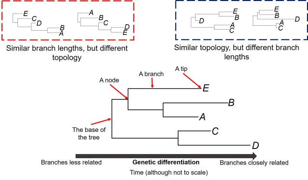
The general anatomy of a phylogenetic tree. A phylogeny describes the relationships of tips (i.e. which are more closely related than others; referred to as the topology), how different these tips are (the length of the branches) and the order they separated in time (separations shown by the nodes). Different trees can share some traits but not others: the red box shows two phylogenetic trees with similar branch lengths (all of the branches are roughly the same) but different topology (the tips connect differently: A and B are together on the left but not on the right, for example). Conversely, two trees can have the same topology, but show differing lengths in the branches of the same tree (blue box). Note that the tips are all in the same positions in these two trees. Typically, it’s easier to read a tree from right to left: the two tips who have branches that meet first are most similar genetically; the longer it takes for two tips to meet along the branches, the less similar they are genetically.

How do we do it?

The parameters

There are a number of parameters that are required for estimating divergence times from a phylogenetic tree. These can be summarised into two distinct categories: the tree model and the substitution model.

The first one of these is relatively easy to explain; it describes the exact relationship of the different samples in our dataset (i.e. the phylogenetic tree). Naturally, this includes the topology of the tree (which determines which divergences times can be estimated for in the first place). However, there is another very important factor in the process: the lengths of the branches within the phylogenetic tree. Branch lengths are related to the amount of genetic differentiation between the different tips of the tree. The longer the branch, the more genetic differentiation that must have accumulated (and usually also meaning that longer time has occurred from one end of the branch to the other). Even two phylogenetic trees with identical topology can give very different results if they vary in their branch lengths (see the above Figure).

The second category determines how likely mutations are between one particular type of nucleotide and another. While the details of this can get very convoluted, it essentially determines how quickly we expect certain mutations to accumulate over time, which will inevitably alter our predictions of how much time has passed along any given branch of the tree.

Calibrating the tree

However, at least one another important component is necessary to turn divergence time estimates into absolute, objective times. An external factor with an attached date is needed to calibrate the relative branch divergences; this can be in the form of the determined mutation rate for all of the branches of the tree or by dating at least one node in the tree using additional information. These help to anchor either the mutation rate along the branches or the absolute date of at least one node in the tree (with the rest estimated relative to this point). The second method often involves placing a time constraint on a particular node of the tree based on prior information about the biogeography of the species (for example, we might know one species likely diverged from another after a mountain range formed: the age of the mountain range would be our constraints). Alternatively, we might include a fossil in the phylogeny which has been radiocarbon dated and place an absolute age on that instead.

Ammonite comic.jpg
Don’t you know it’s rude to ask an ammomite her age?

In regards to the former method, mutation rates describe how fast genetic differentiation accumulates as evolution occurs along the branch. Although mutations gradually accumulate over time, the rate at which they occur can depend on a variety of factors (even including the environment of the organism). Even within the genome of a single organism, there can be variation in the mutation rate: genes, for example, often gain mutations slower than non-coding region.

Although mutation rates (generally in the form of a ‘molecular clock’) have been traditionally used in smaller datasets (e.g. for mitochondrial DNA), there are inherent issues with its assumptions. One is that this rate will apply to all branches in a tree equally, when different branches may have different rates between them. Second, different parts of the genome (even within the same individual) will have different evolutionary rates (like genes vs. non-coding regions). Thus, we tend to prefer using calibrations from fossil data or based on biogeographic patterns (such as the time a barrier likely split two branches based on geological or climatic data).

The analytical framework

All of these components are combined into various analytical frameworks or programs, each of which handle the data in different ways. Many of these are Bayesian model-based analysis, which in short generates hypothetical models of evolutionary history and divergence times for the phylogeny and tests how well it fits the data provided (i.e. the phylogenetic tree). The algorithm then alters some aspect(s) of the model and tests whether this fits the data better than the previous model and repeats this for potentially millions of simulations to get the best model. Although models are typically a simplification of reality, they are a much more tractable approach to estimating divergence times (as well as a number of other types of evolutionary genetics analyses which incorporating modelling).

Molecular dating pipeline
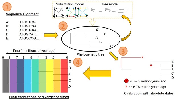
A (believe it or not, simplified) pipeline for estimating divergence times from a phylogeny. 1) We obtain our DNA sequences for our samples: in this example, we’ll see each Sample (A-E) is a representative of a single species. We align these together to make sure we’re comparing the same part of the genome across all of them. 2) We estimate the phylogenetic tree for our samples/species. In a Bayesian framework, this means creating simulation models containing a certain substitution model and a given tree model (containing certain topology and branch lengths). Together, these two models form the likelihood model: we then test how well this model explains our data (i.e. the likelihood of getting the patterns in our data if this model was true). We repeat these simulations potentially hundreds of thousands of times until we pinpoint the most likely model we can get. 3) Using our resulting phylogeny, we then calibrate some parts of it based on external information. This could either be by including a carbon-dated fossil (F) within the phylogeny, or constraining the age of one node based on biogeographic information (the red circle and cross). 4) Using these calibrations as a reference, we then estimated the most likely ages of all the splits in the tree, getting our final dated phylogeny.

Despite the developments in the analytical basis of estimating divergence times in the last few decades, there are still a number of limitations inherent in the process. Many of these relate to the assumptions of the underlying model (such as the correct and accurate phylogenetic tree and the correct estimations of evolutionary rate) used to build the analysis and generate simulations. In the case of calibrations, it is also critical that they are correctly dated based on independent methods: inaccurate radiocarbon dating of a fossil, for example, could throw out all of the estimations in the entire tree. That said, these factors are intrinsic to any phylogenetic analysis and regularly considered by evolutionary biologists in the interpretations and discussions of results (such as by including confidence intervals of estimations to demonstrate accuracy).

Understanding the temporal aspects of evolution and being able to relate them to a real estimate of age is a difficult affair, but an important component of many evolutionary studies. Obtaining good estimates of the timing of divergence of populations and species through molecular dating is but one aspect in building the picture of the history of all organisms, including (and especially) humans.