Conservation biology is frequently referred to as a “crisis discipline“, a status which doesn’t appear to be changing any time soon. Like any response to a crisis, biologists of all walks of life operate under a prioritisation scheme – how can our finite resources be best utilised to save as much biodiversity as possible? This approach requires some knowledge of both current vulnerability and future threat – we need to focus our efforts on those populations and species which are most at-risk of extinction in the near (often immediate) future.
A number of timesbefore on The G-CAT, we’ve discussed the idea of using the frequency of different genetic variants (alleles) within a particular population or species to test a number of different questions about evolution, ecology and conservation. These are all based on the central notion that certain forces of nature will alter the distribution and frequency of alleles within and across populations, and that these patterns are somewhat predictable in how they change.
One particular distinction we need to make early here is the difference between allele frequency and allele identity. In these analyses, often we are working with the same alleles (i.e. particular variants) across our populations, it’s just that each of these populations may possess these particular alleles in different frequencies. For example, one population may have an allele (let’s call it Allele A) very rarely – maybe only 10% of individuals in that population possess it – but in another population it’s very common and perhaps 80% of individuals have it. This is a different level of differentiation than comparing how different alleles mutate (as in the coalescent) or how these mutations accumulate over time (like in many phylogenetic-based analyses).
An example of the difference between allele frequency and identity.In this example (and many of the figures that follow in this post), the circle denote different populations, within which there are individuals which possess either an A gene (blue) or a B gene. Left: If we compared Populations 1 and 2, we can see that they both have A and B alleles. However, these alleles vary in their frequency within each population, with an equal balance of A and B in Pop 1 and a much higher frequency of B in Pop 2. Right: However, when we compared Pop 3 and 4, we can see that not only do they vary in frequencies, they vary in the presence of alleles, with one allele in each population but not the other.
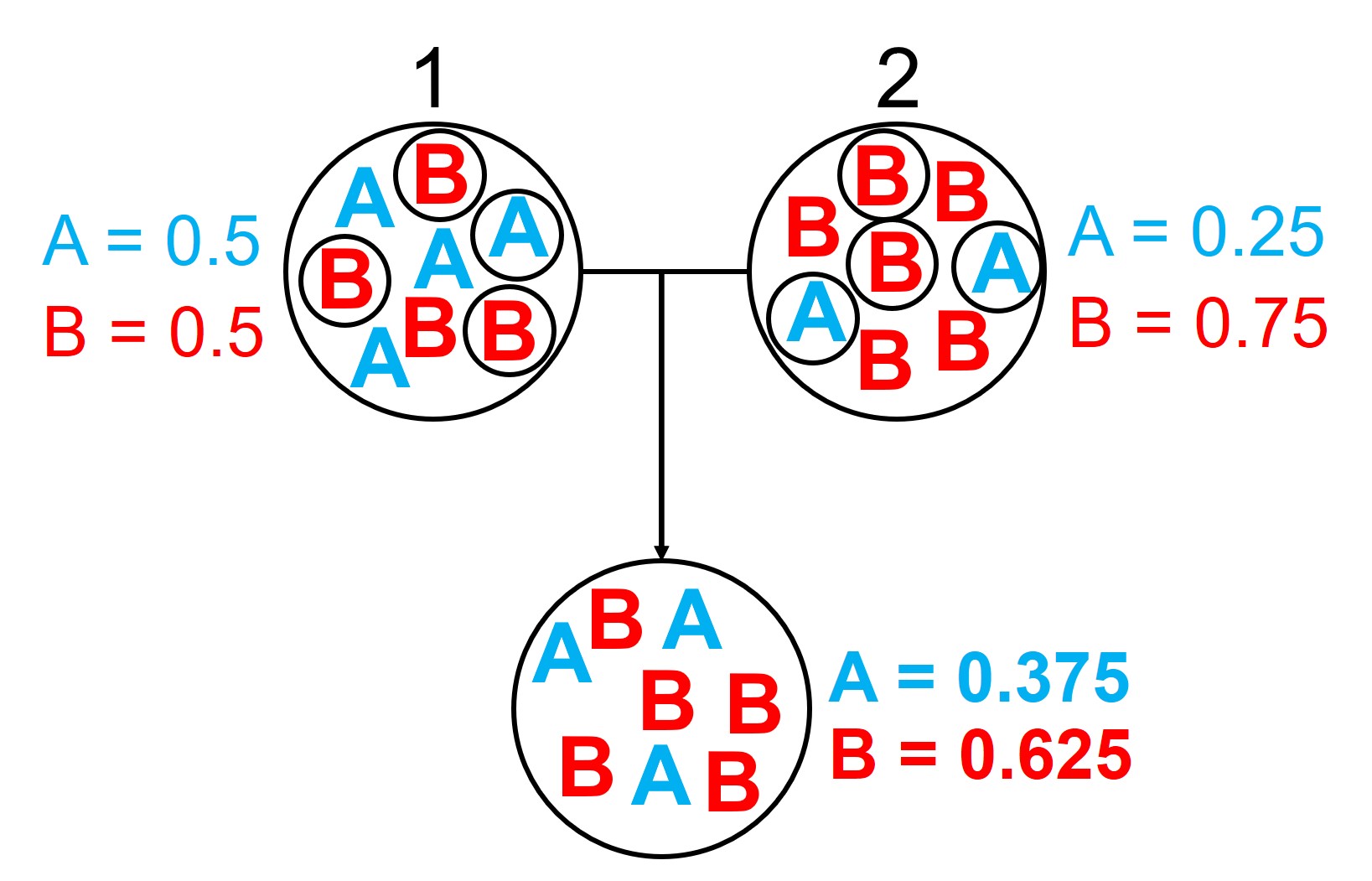
An example of how gene flow across populations homogenises allele frequencies. We start with two initial populations (1 and 2 from above), which have very different allele frequencies. Hybridising individuals across the two populations means some alleles move from Pop 1 and Pop 2 into the hybrid population: which alleles moves is random (the smaller circles). Because of this, the resultant hybrid population has an allele frequency somewhere in between the two source populations: think of like mixing red and blue cordial and getting a purple drink.
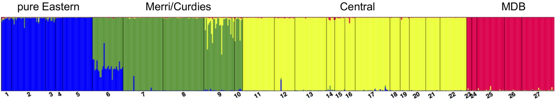
An example of a Structure plot which long-term The G-CAT readers may be familiar with. This is taken from Brauer et al. (2013), where the authors studied the population structure of the Yarra pygmy perch. Each small column represents a single individual, with the colours representing how well the alleles of that individual fit a particular genetic population (each population has one colour). The numbers and broader columns refer to different ‘localities’ (different from populations) where individuals were sourced. This shows clear strong population structure across the 4 main groups, except for in Locality 6 where there is a mixture of Eastern and Merri/Curdies alleles.
Determining genetic bottlenecks and demographic change
A diagram of how allele frequencies change in genetic bottlenecks due to genetic drift. Left: Large circles again denote a population (although across different sequential times), with smaller circle denoting which alleles survive into the next generation (indicated by the coloured arrows). We start with an initial ‘large’ population of 8, which is reduced down to 4 and 2 in respective future times. Each time the population contracts, only a select number of alleles (or individuals) ‘survive’: assuming no natural selection is in process, this is totally random from the available gene pool. Right: We can see that over time, the frequencies of alleles A and B shift dramatically, leading to the ‘extinction’ of Allele B due to genetic drift. This is because it is the less frequent allele of the two, and in the smaller population size has much less chance of randomly ‘surviving’ the purge of the genetic bottleneck.
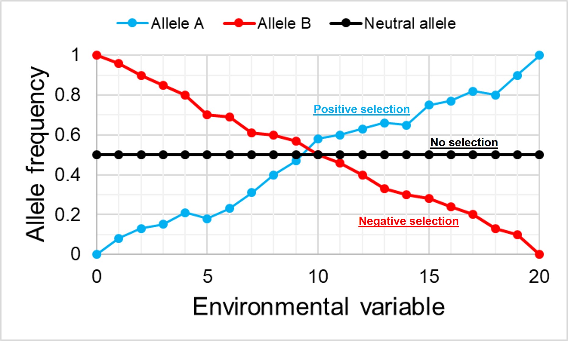
An example of how the frequency of alleles might vary under natural selection in correlation to the environment. In this example, the blue allele A is adaptive and under positive selection in the more intense environment, and thus increases in frequency at higher values. Contrastingly, the red allele B is maladaptive in these environments and decreases in frequency. For comparison, the black allele shows how the frequency of a neutral (non-adaptive or maladaptive) allele doesn’t vary with the environment, as it plays no role in natural selection.
Fixed differences are sometimes used as a type of diagnostic trait for species. This means that each ‘species’ has genetic variants that are not shared at all with its closest relative species, and that these variants are so strongly under selection that there is no diversity at those loci. Often, fixed differences are considered a level above populations that differ by allelic frequency only as these alleles are considered ‘diagnostic’ for each species.
An example of the difference between fixed differences and allelic frequency differences. In this example, we have 5 cats from 3 different species, sequencing a particular target gene. Within this gene, there are three possible alleles: T, A or G respectively. You’ll quickly notice that the T allele is both unique to Species A and is present in all cats of that species (i.e. is fixed). This is a fixed difference between Species A and the other two. Alleles A and G, however, are present in both Species B and C, and thus are not fixed differences even if they have different frequencies.
To distinguish between the two, we often use the overall frequency of alleles in a population as a basis for determining how likely two individuals share an allele by random chance. If alleles which are relatively rare in the overall population are shared by two individuals, we expect that this similarity is due to family structure rather than population history. By factoring this into our relatedness estimates we can get a more accurate overview of how likely two individuals are to be related using genetic information.
The wild world of allele frequency
Despite appearances, this is just a brief foray into the many applications of allele frequency data in evolution, ecology and conservation studies. There are a plethora of different programs and methods that can utilise this information to address a variety of scientific questions and refine our investigations.