Adaptation

From mutation to speciation: the genetics of species formation

July 11, 2018July 11, 2018Sean Buckley4 Comments

The genetics of speciation

Given the strong influence of genetic identity on the process and outcomes of the speciation process, it seems a natural connection to use genetic information to study speciation and species identities. There is a plethora of genetics-based tools we can use to investigate how speciation occurs (both the evolutionary processes and the external influences that drive it). One clear way to test whether two populations of a particular species are actually two different species is to investigate genes related to reproductive isolation: if the genetic differences demonstrate reproductive incompatibilities across the two populations, then there is strong evidence that they are separate species (at least under the Biological Species Concept; see Part One for why!). But this type of analysis requires several tools: 1) knowledge of the specific genes related to reproduction (e.g. formation of sperm and eggs, genital morphology, etc.), 2) the complete and annotated genome of the species (to be able to find and analyse the right genes properly) and 3) a good amount of data for the populations in question. As you can imagine, for people working on non-model species (i.e. ones that haven’t had the same history and detail of research as, say, humans and mice), this can be problematic. So, instead, we can use other genetic information to investigate and suggest patterns and processes related to the formation of new species.

Is reproductive isolation naturally selected for or just a consequence?

A fundamental aspect of studies of speciation is a “chicken or the egg”-type paradigm: does natural selection directly select for rapid reproductive isolation, preventing interbreeding; or as a secondary consequence of general adaptive differences, over a long history of evolution? This might be a confusing distinction, so we’ll dive into it a little more.

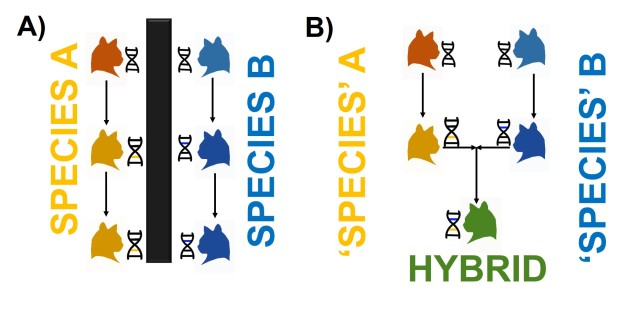
Of the two proposed models of speciation, the by-product of natural selection (the second model) has been the more favoured. Simply put, this expands on Darwin’s theory of evolution that describes two populations of a single species evolving independently of one another. As these become more and more different, both in physical (‘phenotype’) and genetic (‘genotype’) characteristics, there comes a turning point where they are so different that an individual from one population could not reasonably breed with an individual from the other to form a fertile offspring. This could be due to genetic incompatibilities (such as different chromosome numbers), physiological differences (such as changes in genital morphology), or behavioural conflicts (such as solitary vs. group living).

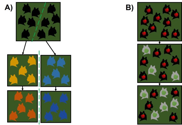
Certainly, this process makes sense, although it is debatable how fast reproductive isolation would occur in a given species (or whether it is predictable just based on the level of differentiation between two populations). Another model suggests that reproductive isolation actually might arise very quickly if natural selection favours maintaining particular combinations of traits together. This can happen if hybrids between two populations are not particularly well adapted (fit), causing natural selection to favour populations to breed within each group rather than across groups (leading to reproductive isolation). Typically, this is referred to as ‘reinforcement’ and predominantly involves isolating mechanisms that prevent individuals across populations from breeding in the first place (since this would be wasted energy and resources producing unfit offspring). The main difference between these two models is the sequence of events: do populations ecologically diverge, and because of that then become reproductively isolated, or do populations selectively breed (enforcing reproductive isolation) and thus then evolve independently?

Reinforcement figure.jpg — An example of reinforcement leading to speciation. A) We start with two populations of a single species (a red fish population and a green fish population), which can interbreed (the arrows). B) Because these two groups can breed, hybrids of the two populations can be formed. However, due to the poor combination of red and green fish genes within a hybrid, they are not overly fit (the red cross). C) Since natural selection doesn’t favour forming hybrids, populations then adapt to selectively breed only with similar fish, reducing the amount of interbreeding that occurs. D) With the two populations effectively isolated from one another, different adaptations specific to each population (spines in red fish, purple stripes in green fish) can evolve, causing them to further differentiate. E) At some point in the differentiation process, hybrids move from being just selectively unfit (as in B)) to entirely impossible, thus making the two populations formal species. In this example, evolution has directly selected against hybrids first, thus then allowing ecological differences to occur (as opposed to the other way around).

Reproductive isolation through DMIs

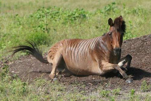
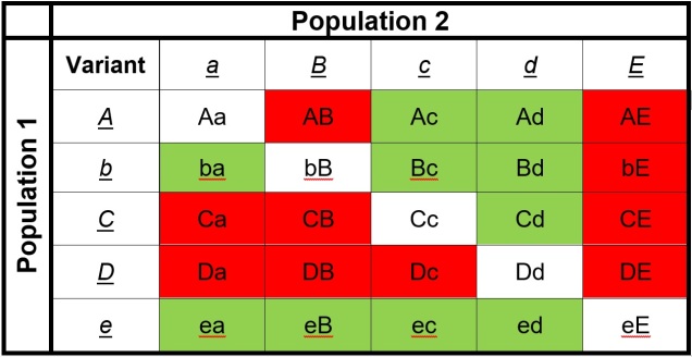
The reproductive incompatibility of two populations (thus making them species) is often intrinsically linked to the genetic make-up of those two species. Some conflicts in the genetics of Population 1 and Population 2 may mean that a hybrid having half Population 1 genes and half Population 2 genes will have serious fitness problems (such as sterility or developmental problems). Dramatic genetic differences, particularly a difference in the number of chromosomes between the two sources, is a significant component of reproductive isolation and is usually to blame for sterile hybrids such as ligers, zorse and mules.

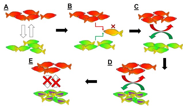
However, subtler genetic differences can also have a strong effect: for example, the unique combination of Population 1 and Population 2 genes within a hybrid might interact with one another negatively and cause serious detrimental effects. These are referred to as “Dobzhansky-Müller Incompatibilities” (DMIs) and are expected to accumulate as the two populations become more genetically differentiated from one another. This can be a little complicated to imagine (and is based upon mathematical models), but the basis of the concept is that some combinations of gene variants have never, over evolutionary history, been tested together as the two populations diverge. Hybridisation of these two populations suddenly makes brand new combinations of genes, some of which may be have profound physiological impacts (including on reproduction).

DMI figure — An example of how Dobzhansky-Müller Incompatibilities arise, adapted from Coyne & Orr (2004). We start with an initial population (center top), which splits into two separate populations. In this example, we’ll look at how 5 genes (each letter = one gene) change over time in the separate populations, with the original allele of the gene (lowercase) occasionally mutating into a new allele (upper case). These mutations happen at random times and in random genes in each population (the red letters), such that the two become very different over time. After a while, these two populations might form hybrids; however, given the number of changes in each population, this hybrid might have some combinations of alleles that are ‘untested’ in their evolutionary history (see below). These untested combinations may cause the hybrid to be infertile or unviable, making the two populations isolated species.

DMI table — The list of ‘untested’ genetic combinations from the above example. This table shows the different combinations of each gene that could be made in a hybrid if these two populations interbred. The red cells indicate combinations that have never been ‘tested’ together; that is, at no point in the evolutionary history of these two populations were those two particular alleles together in the same individual. Green cells indicate ones that were together at some point, and thus are expected to be viable combinations (since the resultant populations are obviously alive and breeding).

How can we look at speciation in action?

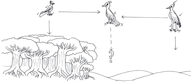
We can study the process of speciation in the natural world without focussing on the ‘reproductive isolation’ element of species identity as well. For many species, we are unlikely to have the detail (such as an annotated genome and known functions of genes related to reproduction) required to study speciation at this level in any case. Instead, we might choose to focus on the different factors that are currently influencing the process of speciation, such as how the environmental, demographic or adaptive contexts of populations plays a role in the formation of new species. Many of these questions fall within the domain of phylogeography; particularly, how the historical environment has shaped the diversity of populations and species today.

Phylogeo of speciation — An example of the interplay between speciation and phylogeography, taken from Reyes-Velasco et al. (2018). They investigated the phylogeographic history of several different groups of species within the frog genus Ptychadena; in this figure, we can see how the different species (indicated by the colours and tree on the left) relate to the geography of their habitat (right).

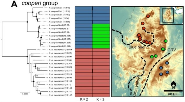
A variety of different analytical techniques can be used to build a picture of the speciation process for closely related or incipient species. A good starting point for any speciation study is to look at how the different study populations are adapting; is there evidence that natural selection is pushing these populations towards different genotypes or ecological niches? If so, then this might be a precursor for speciation, and we can build on this inference with other complementary analyses.

For example, estimating divergence times between populations can help us suggest whether there has been sufficient time for speciation to occur (although this isn’t always clear cut). Additionally, we could estimate the levels of genetic hybridisation (‘introgression’) between two populations to suggest whether they are reasonably isolated and divergent enough to be considered functional species.

The future of speciation genomics

Although these can help answer some questions related to speciation, new tools are constantly needed to provide a clearer picture of the process. Understanding how and why new species are formed is a critical aspect of understanding the world’s biodiversity. How can we predict if a population will speciate at some point? What environmental factors are most important for driving the formation of new species? How stable are species identities, really? These questions (and many more) remain elusive for a wide variety of life on Earth.

Of birds and bees: where do species come from?

July 4, 2018July 4, 2018Sean Buckley9 Comments

This is Part 2 of a four part miniseries on the process of speciation: how we get new species, how we can see this in action, and the end results of the process. This week we’re taking a look at how new species are formed from natural selection. For Part 1, on the identity and concept of the species, click here.

The Origin of Species

Despite Darwin’s scientifically ground-breaking revelations over 150 years ago, the truth of the origin of species has remained a puzzling and complex question in biology. While the fundamental concepts of Darwin’s theory remain heavily supported – that groups which become separated from one another and undergo differing evolutionary pathways through natural selection may over time form new species – the mechanisms leading to this are mysterious. Even though the heritable component of evolution (DNA) was not uncovered for a hundred years after publishing ‘On the Origin of Species’, Darwin’s theory can largely explain many patterns of the formation of species on Earth.

The population-speciation continuum

The understanding that groups that are separated progress into species through differential adaptation leads to a phenomenon as the ‘speciation continuum’: all populations exist at some point on the continuum, with those that are most differentiated (i.e. most progressed) are distinct species, whereas those least differentiated are closely related or the same population. Whether or not populations progress along this continuum, and how fast this progression happens, depends on the difference in selective pressure and speed of evolution in the populations. Even if two populations are physically separated, they might not necessarily form new species if the separation is too short-term or if they do not evolve in different ways. Even if they do differentially evolve, whether or not they develop reproductive isolation is not always consistent.

Speciation continuum figure — A vague diagram of the population-speciation continuum. In this figure, we have two different organisms (Taxa 1 and Taxa 2) and we’re comparing their genetic similarity/differences (the grey arrow). At the bottom left of the chart, there are very few genetic differences between the two, likely indicated that they are from the same population (or closely related e.g. siblings). As we progress towards the upper left, the two start to diverge from one another, first to different populations of the same species, different subspecies of the same overarching species, and eventually becoming so different that they must be new species (i.e. are genetically incompatible and thus reproductively isolated). Exactly where this cut-off is a bit of a grey area (the species boundary) and is unlikely to be consistent across species.

Furthermore, how these populations are changing may affect the rate or success of speciation: if the traits that evolve differently across the population also cause them to be unable to breed, then they may quickly become reproductively isolated and thus new species. For example, Momigliano et al. (2017) demonstrated the fastest known rate of speciation (within 3000 generations) in a marine vertebrate in a species of flounders. Flounders that adapted to a higher salinity environment became reproductively isolated from their sister population as their sperm could not tolerate the high salinity conditions (directly preventing breeding and causing reproductive isolation). This strong and rapid selection to an environment, and its subsequent selection on reproductive ability, was cutely described as a “magic trait”.

Modes of speciation

Darwin’s model of speciation describes what is called “allopatric speciation”, whereby physical separation of populations by some form of barrier (often attributed to changes such as climatic shifts, mountain range formations or island separation) isolates populations which then independently evolve until they reach a point of differentiation where they can no longer interbreed. Thus, they are now separate species (based on the Biological Species Concept, anyway). Allopatric speciation has traditionally believed to be the most common process of speciation, and is consistently used as the model for teaching and understanding speciation.

While this physical separation is the strongest and most immediately obvious method of speciation, other forms without geographic barriers have been documented. “Sympatric speciation” involves speciation events where there are no apparent geographical barriers that separate populations: instead, other factors may be driving their divergence from one another. This can relate to different microenvironments within the same area, where one population migrates and adapts to an environment which excludes the other population. This is referred to as “ecological speciation” and has been particularly noted within lake fish radiating into different habitats. There are a number of other mechanisms by which sympatric speciation could also occur, however, including temporal isolation (e.g. different flowering times in plants), sexual selection (e.g. a mutation leads to a new physiology that is more attractive to others with that physiology) or polyploidy (e.g. a ‘mutation’ causes an organism to have multiple copies of its genome, making it effectively reproductively isolated from its neighbours due to incompatible sex cells).

Allopatric vs sympatric speciation — Representations of allopatric and sympatric speciation using our friends the fruit-eating cats. A) An example of allopatric speciation. Similar to how we’ve seen it before, a geographic barrier (the dashed green line) separates the ancestral species in two; each of these groups then evolve in different directions based on the different environmental pressures of each zone. After enough divergence, these two groups become reproductively isolated from one another and thus are different species. B) An example of sympatric speciation. We start with a single species of red apple eating cats, which form one contiguous group. A mutation within the group produces a new type of fruit-eating cat; one that feeds on green apples (grey cats). Because these feed on a different food source, they move into a different part of the environment, associating with other green apple-eating cats and less with red apple-eating cats. Over time, and with strong enough selection for apple preferences, these two types may become different species.

Sympatric speciation has received a great deal of controversy, due to the fact that some levels of gene flow could occur across the two populations with relative ease (compared to allopatric populations). This gene flow should cause the two populations to reconnect and prevent each population from evolving differently from one another (as changes in one population’s gene pool will be introduced into the other). Speciation with gene flow has been shown for some species, based on the idea that the pressure of natural selection (i.e. being adapted to the right habitat) is much stronger than the level of gene flow (i.e. the introduction of non-adapted genes from the other population), so the two populations still diverge genetically.

Gene flow across populations (through hybridisation) will balance out the different allele frequencies of the two gene pools, preventing adaptive alleles from moving towards fixation as per the standard natural selection process. While the effect of gene flow might slow the process, taking longer for the populations to diverge to the species level, speciation can still be achieved. Thus, the balance of gene flow and adaptive divergence is critical in determining whether ecological speciation is possible.

Sympatric speciation figure — A slightly more convoluted example of sympatric speciation. A) We start with a single species of small orange cats (top row), which can share readily share genes with one another. A mutation within the species creates a new type of cat; one that is much larger and has tufted ears. Although there are somewhat morphologically distinct from one another, they’re still genetically similar enough to continue to breed and share genes across the two types. However, with the big size comes a new ecological niche and these big cats differentially evolve to be grey (to hide better from their new bigger prey, perhaps) whilst the non-mutated group stays the same size and colour. Because large grey cats will preferentially breed with other large grey cats and not with small orange cats, this group genetically diverges from the ancestor to form a new species. B) A representation of the genetic changes between the two groups over time. The figure shows the genome (the grey bar) of the cat; the y-axis is the level of genetic differentiation between the two (measured as Fst). The different coloured sections represent specific genes within the genome, whilst the dashed line represents the average Fst across the whole genome. At initial divergence (top), there is little difference between the two. However, as the new big cats form and evolve, we can see the average Fst increase, with strong peaks around particular genes (blue and green; those related to the changes in physiology). As the two groups continue to diverge, this average raises even higher until genetic changes cause the reproduction-related genes (red and yellow) to become too different to allow for hybridisation, making the two species reproductively isolated (the red X in A)).

The reality of species

While the distinction between divergent populations and species might be a complex one, development in genomic technologies and greater understanding of evolutionary patterns is helping us uncover the real origin of species. And while species might not be as concrete a concept as one might expect, understanding the processes that generate new species and diversity is critical for understanding the diversity within nature that we see today, and also the potential diversity for the future (and why protecting said diversity is important!).

What is a species, anyway?

June 27, 2018June 26, 2018Sean Buckley9 Comments

This is Part 1 of a four part miniseries on the process of speciation; how we get new species, how we can see this in action, and the end results of the process. This week, we’ll start with a seemingly obvious question: what is a species?

The definition of a ‘species’

‘Species’ are a human definition of the diversity of life. When we talk about the diversity of life, and the myriad of creatures and plants on Earth, we often talk about species diversity. This might seem glaringly obvious, but there’s one key issue: what is a species, anyway? While we might like to think of them as discrete and obvious groups (a dog is definitely not the same species as a cat, for example), the concept of a singular “species” is actually the result of human categorisation.

In reality, the diversity of life is spread across a huge spectrum of differentiation: from things which are closely related but still different to us (like chimps), to more different again (other mammals), to hardly relatable at all (bacteria and plants). So, what is the cut-off for calling something a species, and not a different genus, family, or kingdom? Or alternatively, at what point do we call a specific sub-group of a species as a sub-species, or another species entirely?

This might seem like a simple question: we look at two things, and they look different, so they must be different species, right? Well, of course, nature is never simple, and the line between “different” and “not different” is very blurry. Here’s an example: consider that you knew nothing about the history, behaviour or genetics of dogs. If you simply looked at all the different breeds of dogs on Earth, you might suggest that there are hundreds of species of domestic dogs. That seems a little excessive though, right? In fact, the domestic dog, Eurasian wolf, and the Australian dingo are all the same species (but different subspecies, along with about 38 others…but that’s another issue altogether).

Dogs — Morphology can be misleading for identifying species. In this example, we have A) a dog, B) also a dog, C) still a dog, D) yet another dog, and E) not a dog. For the record, **A-D** are all Canis lupus of some variety; A and B are domestic dogs (Canis lupus familiaris), C is a dingo (Canis lupus dingo) and D is a grey wolf (Canis lupus lupus). E, however, is the Ethiopian wolf, Canis simensis.

How do we describe species?

This method of describing species based on how they look (their morphology) is the very traditional approach to taxonomy. And for a long time, it seemed to work…until we get to more complex scenarios like the domestic dog. Or scenarios where two species look fairly similar, but in reality have evolved entirely differently for a very, very long time. Or groups which look close to more than one other species. So how do we describe them instead?

Cats and foxes — A), a fox. B), a cat. C), a foxy cat? A catty fox? A cat-fox hybrid? Something unrelated to cat or a fox?

Believe it or not, there are dozens of ways of deciding what is a species and what isn’t. In Speciation (2004), Coyne & Orr count at least 25 different reported Species Concepts that had been suggested within science, based on different requirements such as evolutionary history, genetic identity, or ecological traits. These different concepts can often contradict one another about where to draw the line between species…so what do we use?

The Biological Species Concept (BSC)

The most commonly used species concept is called the Biological Species Concept (BSC), which denotes that “species are groups of interbreeding natural populations that are reproductively isolated from other such groups” (Mayr, 1942). In short, a population is considered a different species to another population if an individual from one cannot reliably breed to form fertile, viable offspring with an individual from the other. We often refer to this as “reproductive isolation.” It’s important to note that reproductive isolation doesn’t mean they can’t breed at all: just that the hybrid offspring will not live a healthy life and produce its own healthy offspring.

For example, a horse and zebra can breed to produce a zorse, however zorse are fundamentally infertile (due to the different number of chromosomes between a horse and a zebra) and thus a horse is a different species to a zebra. However, a German Shepherd and a chihuahua can breed and make a hybrid mutt, so they are the same species.

You might naturally ask why reproductive isolation is apparently so important for deciding species. Most directly, this means that groups don’t share gene pools at all (since genetic information is introduced and maintained over time through breeding events), which causes them to be genetically independent of one another. Thus, changes in the genetic make-up of one species shouldn’t (theoretically) transfer into the gene pool of another species through hybrids. This is an important concept as the gene pool of a species is the basis upon which natural selection and evolution act: thus, reproductively isolated species may evolve in very different manners over time.

RI example — An example of how reproductive isolation maintains genetic and evolutionary independence of species. In A), our cat groups are robust species, reproductively isolated from one another (as shown by the black box). When each species undergoes natural selection and their genetic variation changes (colour changes on the cats and DNA), these changes are kept within each lineage. This contrasts to B), where genetic changes can be transferred between species. Without reproductive isolation, evolution in the orange lineage and the blue lineage can combine within hybrids, sharing the evolutionary pathways of both ancestral species.

Pitfalls of the BSC

Just because the BSC is the most used concept doesn’t make it infallible, however. Many species on Earth don’t easily demonstrate reproductive isolation from one another, nor does the concept even make sense for asexually reproducing species. If an individual reproduced solely asexually (like many bacteria, or even some lizards), then by the BSC definition every individual is an entirely different species…which seems a little excessive. Even in sexually reproducing organisms, it can be hard to establish reproductive isolation, possibly because the species never come into contact physically.

This raises the debate of whether two species could, let alone will, hybridise in nature, which can be difficult to determine. And if two species do produce hybrid offspring, assessing their fertility or viability can be difficult to detect without many generations of breeding and measurements of fitness (hybrids may not be sustainable in nature if they are not well adapted to their environment and thus the two species are maintained as separate identities).

Hybrid birds — An example of unfit hybrids causing effective reproductive isolation. In this example, we have two different bird species adapted to very different habitats; a smaller, long-tailed bird (left) adapted to moving through dense forest, and a large, longer-legged bird (right) adapted to traversing arid deserts. When (or if) these two species hybridised, the resultant offspring would be middle of the road, possessing too few traits to be adaptive in either the forest or the desert and no fitting intermediate environment available. Measuring exactly how unfit this hybrid would be is a difficult task in establishing species boundaries.

Integrative taxonomy

To try and account for the issues with the BSC, taxonomists try to push for the usage of “integrative taxonomy”. This means that species should be defined by multiple different agreeing concepts, such as reproductive isolation, genetic differentiation, behavioural differences, and/or ecological traits. The more traits that can separate the two, the greater support there is for the species to be separated: if they disagree, then more information is needed to determine exactly whether or not that should be called different species. Debates about taxonomy are ongoing and are likely going to be relevant for years to come, but form critical components of understanding biodiversity, patterns of evolution, and creating effective conservation legislation to protect endangered or threatened species (for whichever groups we decide are species).

The direction of evolution: divergence vs. convergence

June 6, 2018June 7, 2018Sean Buckley6 Comments

Direction of evolution

We’ve talked previously on The G-CAT about how the genetic underpinning of certain evolutionary traits can change in different directions depending on the selective pressure it is under. Particularly, we can see how the frequency of different alleles might change in one direction or another, or stabilise somewhere in the middle, depending on its encoded trait. But thinking bigger picture than just the genetics of one trait, we can actually see that evolution as an entire process works rather similarly.

Divergent evolution

The classic view of the direction of evolution is based on divergent evolution. This is simply the idea that a particular species possess some ancestral trait. The species (or population) then splits into two (for one reason or another), and each one of these resultant species and populations evolves in a different way to the other. Over time, this means that their traits are changing in different directions, but ultimately originate from the same ancestral source.

Evidence for divergent evolution is rife throughout nature, and is a fundamental component of all of our understanding of evolution. Divergent evolution means that, by comparing similar traits in two species (called homologous traits), we can trace back species histories to common ancestors. Some impressive examples of this exist in nature, such as the number of bones in most mammalian species. Humans have the same number of neck bones as giraffes; thus, we can suggest that the ancestor of both species (and all mammals) probably had a similar number of neck bones. It’s just that the giraffe lineage evolved longer bones whereas other lineages did not.

Homology figure — A diagrammatic example of homologous structures in ‘hand’ bones. The coloured bones demonstrate how the same original bone structures have diverged into different forms. Source: BiologyWise.

Convergent evolution

But of course, evolution never works as simply as you want it to, and sometimes we can get the direct opposite pattern. This is called convergent evolution, and occurs when two completely different species independently evolve very similar (sometimes practically identical) traits. This is often caused by a limitation of the environment; some extreme demand of the environment requires a particular physiological solution, and thus all species must develop that trait in order to survive. An example of this would be the physiology of carnivorous marsupials like Tasmanian devils or thylacines: despite being in another Class, their body shapes closely resemble something more canid. Likely, the carnivorous diet places some constraints on physiology, particularly jaw structure and strength.

Convergent evol intelligence — A surprising example of convergent evolution is cognitive ability in apes and some bird groups (e.g. corvids). There’s plenty of other animal groups more related to each of these that don’t demonstrate the same level of cognitive reasoning (based on the traits listed in the centre): thus, we can conclude that cognition has evolved twice in very, very different lineages. Source: Emery & Clayton, 2004.

A more dramatic (and potentially obvious) example of convergent evolution would be wings and the power of flight. Despite the fact that butterflies, bees, birds and bats all have wings and can fly, most of them are pretty unrelated to one another. It seems much more likely that flight evolved independently multiple times, rather than the other 99% of species that shared the same ancestor lost the capacity of flight.

Parallel evolution

Sometimes convergent evolution can work between two species that are pretty closely related, but still evolved independently of one another. This is distinguished from other categories of evolution as parallel evolution: the main difference is that while both species may have shared the same start and end point, evolution has acted on each one independent of the other. This can make it very difficult to diagnose from convergent evolution, and is usually determined by the exact history of the trait in question.

Parallel evolution is an interesting field of research for a few reasons. Firstly, it provides a scenario in which we can more rigorously test expectations and outcomes of evolution in a particular environment. For example, if we find traits that are parallel in a whole bunch of fish species in a particular region, we can start to look at how that particular environment drives evolution across all fish species, as opposed to one species case studies.

Marsupial handedness.jpg — Here’s another weird example; different populations of marsupials (particularly kangaroos and wallabies) show preferential handedness depending on where the population is. That is, different populations of different species of marsupials shows parallel evolution of handedness, since they’re related to one another but have evolved it independently of the other species. Source: Giljov et al. (2015).

Following from that logic, it is then important to question the mechanisms of parallelism. From a genetic point of view, do these various species use the same genes (and genetic variants) to produce the same identical trait? Or are there many solutions to the selective question in nature? While these questions are rather complicated, and there has been plenty of evidence both for and against parallel genetic underpinning of parallel traits, it seems surprisingly often that many different genetic combinations can be used to get the same result. This gives interesting insight into how complex genetic coding of traits can be, and how creative and diverse evolution can be in the real world.

Where is evolution going?

Cat phylogeny — An example of all three types of evolutionary trajectory in a single phylogeny of cats (you know how we do it here at The G-CAT). This phylogeny consists of two distinct genera; one with one species (P. aliquam) and another of three species (the red box indicates their distance). Our species have three main physical traits: coat colour, ear tufts and tail shape. At the ancestral nodes of the tree, we can see what the ancestor of these species looked like for these three traits. Each of these traits has undergone a different type of evolution. The tufts on the ears are the result of divergent evolution, since F. tuftus evolved the trait differently to its nearest relative, F. griseo. Contrastingly, the orange coat colour of F. tuftus and P. aliquam are the result of convergent evolution: neither of these species are very closely related (remembering the red box) and evolved orange coats independently of one another (since their ancestors are grey). And finally, the fluffy tails of F. hispida and F. griseo can be considered parallel evolution, since they’re similar evolutionarily (same genus) but still each evolved tail fluff independently (not in the ancestor). This example is a little convoluted, but if you trace the history of each trait in the phylogeny you can more easily see these different patterns.

So, where is evolution going for nature? Well, the answer is probably all over the place, but steered by the current environmental circumstances. Predicting the evolutionary impacts of particular environmental change (e.g. climate change) is exceedingly difficult but a critical component of understanding the process of evolution and the future of species. Evolution continually surprises us with creative solution to complex problems and I have no doubt new mysteries will continue to be thrown at us as we delve deeper.

All the world in the palm of your hand: whole genome sequencing for evolution and conservation

May 30, 2018Sean Buckley4 Comments

Building an entire genome

If bigger is better, then biggest is best. Having the genome of a particular study species fully sequenced allows us to potentially look at all of the genetic variation in the entire gene pool: but how do we sequence the entirety of the genome? And what are the benefits of having a whole genome to refer to?

Whole genome assembly — A very, very simplified overview of whole genome sequencing. Similar to other genomic technologies, we start by fragmenting the genome into much smaller, easier to sequence parts (reads). We then use a computer algorithm which pieces these reads together into a consecutive sequence based on overlapping DNA sequence (like building a chain out of Lego blocks). From this assembled genome, we can then attach annotations using information from other species’ genomes or genetic studies, which can correlate a particular sequence to a gene, a function of that gene, and the resultant protein from these gene (although not always are all of these aspects included).

Well, assembling the whole genome of an organism for the first time is a very tricky process. It involves taking DNA sequence from only a few individuals, breaking them down into smaller fragments and multiplying these fragments into the billions (moreorless the same process used in other genomics technologies: the real difference is that we need the full breadth of the genome so that we don’t miss any spaces). From these fragments, we use a complex computer algorithm which builds up a consensus sequence like a Lego tower; by finding parts of sequences which overlap, the software figures out which pieces connect to one another. Hopefully, we eventually end up with one very long continuous sequence; the genome! Sometimes, we might end with a few very large blocks (called contigs), but this is also useful for analyses (correlated with how many/big blocks there are). With this full genome, we use information from other more completed genomes (such as those from model species like humans, mice or even worms) to figure out which sections of the genome relate to specific genes. We can then annotate these sections by labelling them as clear genes, complete with start and end point, and attach a particular physical function of that gene.

The benefits of whole genomes

Having an entire genome as a reference is an extremely helpful tool in conservation and evolutionary studies. The first, and perhaps most obvious benefit, is the sheer scale of the data we can use. By having the entirety of the genome available, we can use potentially billions of base pairs of sequence in our genetic analyses (for reference, the human genome is >3 billion base pairs long). Even if we don’t sequence the full genome for all of our samples, having a reference genome as basis for assembly our reduced datasets significantly improves the quantity and quality of sequences we can use.

Another very important benefit is the ability to prescribe function in our studies. Many of our processes for obtaining data, even for genomic technologies, use random and anonymous fragments of the genome. Although this is a cost-effective way to obtain a very large amount of data, it unfortunately means that we often have no idea which part of the genome our sequences came from. This means that we don’t know which sequences relate to specific genes, and even if we did we would have no idea what those genes are or do! But with an annotated genome, we can take even our fragmented sequence and check it against the genome and find out what genes are present.

Understanding adaptation

Based on that, it seems pretty obvious about exactly how having an annotated genome can help us in studies of adaptation. Knowing the functional aspect of our genetic data allows us to more directly determine how evolution is happening in nature; instead of only being able to say that two species are evolving differently from one another, for example, we can explicitly look at how they are evolving. Is one evolving tolerance to hotter temperatures? Are they evolving different genes to handle different diets? Are they evolving in response to an external influence, like a viral outbreak or changing climate? What are the physiological consequences of these changes? These questions are critical in understanding past and future evolution, and full genome analysis allows us to delve into them much deeper.

Manhattan plot example — A (slightly edited) figure of full genome comparisons between domestic dogs and wild wolves by Axelsson *et al.* (2013), with the aim of understanding the evolutionary changes associated with domestication. For avid readers, this figure probably looks familiar. This figure compares the genetic differentiation across the entire genome between dogs and wolves, with some sections of the genome (circled) showing clear differences. As there is an annotated dog genome, the authors then delved into these genes to understand the functional differences between the two. By comparing their genetic differences to functional genes, the authors can more explicitly suggest mechanisms or changes associated with the domestication process (such as adaptation to a starch-heavy and human-influenced diet).

This includes allowing us to better understand how adaptation actually works in nature. As we’ve discussed before, more traditional studies often assumed that single, or very few, genes were responsible for allowing a species to adapt and change, and that these genes had very strong effects on their physiology. But what we see far more often is polygenic adaptation; small changes in a very large number of genes which, combined together, allow the species to adapt and evolve. By having the entirety of the genome available, we are much more likely to capture all of the genes that are under natural selection in a particular population or species, painting a clearer picture of their evolutionary trajectory.

Understanding demography

The much larger dataset of full genomes is also important for understanding the non-adaptive parts of evolution; the demographic history. Given that selectively neutral impacts (e.g. reductions in population size) are likely to impact all of the genes in the gene pool somewhat equally, having a full genome allows us to more accurately infer the demographic state and historical patterns of species.

For both adaptive and non-adaptive variation, it is also important to consider what we call linkage disequilibrium. Genetic sequences that are physically close to each other in the genome will often be inherited together due to the imprecision of recombination (a fairly technical process, so I won’t delve into this): what this can mean is that if a gene is under very strong selection, then sequences around this gene will also look like they’re under selection too. This can give falsely positive adaptive genes (i.e. sequences that look like genes under selection but are just linked to a gene that is) or can interfere with demographic analyses (since they often assume no selection, or linkage to selection, on the sequences used). With a whole genome, we can actually estimate how far away a base pair has to be before it’s not linked anymore; we call these linkage blocks, and they’re very useful additions to analyses.

Linkage_example — An example of linkage as a process. We start with a particular sequence (top); during recombination, this sequence may randomly break and rearrange into different parts. In this example, I’ve simulated four different ‘breaks’ (dashed coloured lines) due to recombination. Each of these breaks leads to two separate blocks of fragments; for example, the break at the blue line results in the second two sequence blocks (middle). If we focus on one target base pair in the sequence (golden A), then we can see in some fragments it remains with certain bases, but sometimes it gets separated by the break. If we compare how often the golden A is in the same block (i.e. is co-inherited) as each of the other bases, across all 4 breaks, then we see that the bases that are closest to it (the golden A is represented by the golden bar) are almost always in the same block. This makes sense: the further away a base is from our target, the more likely that there will be a break between it. This is shown in the frequency distributions at the bottom: the left figure shows the actual frequencies of co-inheritance (i.e. linkage) using the top example and those 4 breaks. The right figure shows a more realistic depiction of how linkage looks in the genome; it rapidly decays as we move away from the target (although the width and rate of this can vary).

Improving conservation management

In a similar fashion to demography, full genome datasets can improve our estimates of relatedness and pedigrees in captive breeding programs. The massive scale of whole genomes allows us to more easily trace the genealogical history of individuals, allowing us to assign parents more accurately. This also helps with our estimations of genetic relatedness, arguably the most critical aspect of genetic-based breeding programs. This is particularly helpful for species with tricky mating patterns, such as polyamory, brood spawning or difficult to track organisms.

The way forwards

While many non-model species are still lacking in the available genomic information, whole genomes are progressively being sequenced for more and more species. As this astronomical dataset grows, our ability to investigate, discover and test theories about evolution, natural selection and conservation will also improve. Many projects already exist which aim specifically to increase the number of whole genomes available for certain taxonomic groups such as birds and bats: these will no doubt prove to be invaluable resources for future studies.

The G-cat

Dive head-first into the science of conservation, ecology, evolution and genetics