The G-cat

Bringing alleles back together: applications of coalescent theory

November 9, 2018Sean Buckley7 Comments

Coalescent theory

A recurring analytical method, both within The G-CAT and the broader ecological genetic literature, is based on coalescent theory. This is based on the mathematical notion that mutations within genes (leading to new alleles) can be traced backwards in time, to the point where the mutation initially occurred. Given that this is a retrospective, instead of describing these mutation moments as ‘divergence’ events (as would be typical for phylogenetics), these appear as moments where mutations come back together i.e. coalesce.

There are a number of applications of coalescent theory, and it is particularly fitting process for understanding the demographic (neutral) history of populations and species.

Mathematics of the coalescent

Before we can explore the multitude of applications of the coalescent, we need to understand the fundamental underlying model. The initial coalescent model was described in the 1980s, built upon by a number of different ecologists, geneticists and mathematicians. However, John Kingman is often attributed with the formation of the original coalescent model, and the Kingman’s coalescent is considered the most basic, primal form of the coalescent model.

From a mathematical perspective, the coalescent model is actually (relatively) simple. If we sampled a single gene from two different individuals (for simplicity’s sake, we’ll say they are haploid and only have one copy per gene), we can statistically measure the probability of these alleles merging back in time (coalescing) at any given generation. This is the same probability that the two samples share an ancestor (think of a much, much shorter version of sharing an evolutionary ancestor with a chimpanzee).

Normally, if we were trying to pick the parents of our two samples, the number of potential parents would be the size of the ancestral population (since any individual in the previous generation has equal probability of being their parent). But from a genetic perspective, this is based on the genetic (effective) population size (Ne), multiplied by 2 as each individual carries two copies per gene (one paternal and one maternal). Therefore, the number of potential parents is 2Ne.

Constant Ne and coalescent prob — A graph of the probability of a coalescent event (i.e. two alleles sharing an ancestor) in the immediately preceding generation (i.e. parents) relatively to the size of the population. As one might expect, with larger population sizes there is low chance of sharing an ancestor in the immediately prior generation, as the pool of ‘potential parents’ increases.

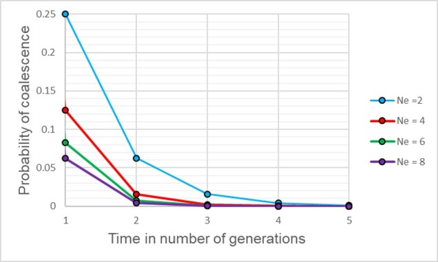
If we have an idealistic population, with large Ne, random mating and no natural selection on our alleles, the probability that their ancestor is in this immediate generation prior (i.e. share a parent) is 1/(2Ne). Inversely, the probability they don’t share a parent is 1 − 1/(2Ne). If we add a temporal component (i.e. number of generations), we can expand this to include the probability of how many generations it would take for our alleles to coalesce as (1 – (1/2Ne))^t-1 x 1/2Ne.

Variable Ne and coalescent probs — The probability of two alleles sharing a coalescent event back in time under different population sizes. Similar to above, there is a higher probability of an earlier coalescent event in smaller populations as the reduced number of ancestors means that alleles are more likely to ‘share’ an ancestor. However, over time this pattern consistently decreases under all population size scenarios.

Although this might seem mathematically complicated, the coalescent model provides us with a scenario of how we would expect different mutations to coalesce back in time if those idealistic scenarios are true. However, biology is rarely convenient and it’s unlikely that our study populations follow these patterns perfectly. By studying how our empirical data varies from the expectations, however, allows us to infer some interesting things about the history of populations and species.

Testing changes in Ne and bottlenecks

One of the more common applications of the coalescent is in determining historical changes in the effective population size of species, particularly in trying to detect genetic bottleneck events. This is based on the idea that alleles are likely to coalesce at different rates under scenarios of genetic bottlenecks, as the reduced number of individuals (and also genetic diversity) associated with bottlenecks changes the frequency of alleles and coalescence rates.

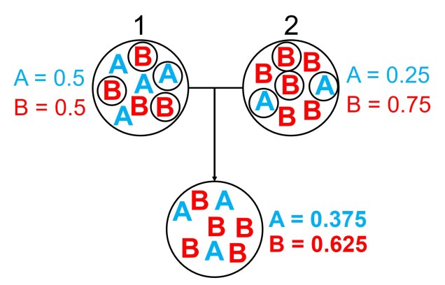
For a set of k different alleles, the rate of coalescence is determined as k(k – 1)/4Ne. Thus, the coalescence rate is intrinsically linked to the number of genetic variants available: Ne. During genetic bottlenecks, the severely reduced Ne gives the appearance of coalescence rate speeding up. This is because alleles which are culled during the bottleneck event by genetic drift causes only a few (usually common) alleles to make it through the bottleneck, with the mutation and spread of these alleles after the bottleneck. This can be a little hard to think of, so the diagram below demonstrates how this appears.

Bottleneck test figure.jpg — A diagram of how the coalescent can be used to detect bottlenecks in a single population (centre). In this example, we have contemporary population in which we are tracing the coalescence of two main alleles (red and green, respectively). Each circle represents a single individual (we are assuming only one allele per individual for simplicity, but for most animals there are up to two). Looking forward in time, you’ll notice that some red alleles go extinct just before the bottleneck: they are lost during the reduction in Ne. Because of this, if we measure the rate of coalescence (right), it is much higher during the bottleneck than before or after it. Another way this could be visualised is to generate gene trees for the alleles (left): populations that underwent a bottleneck will typically have many shorter branches and a long root, as many branches will be ‘lost’ by extinction (the dashed lines, which are not normally seen in a tree).

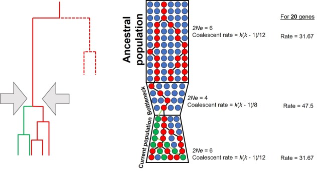
This makes sense from theoretical perspective as well, since strong genetic bottlenecks means that most alleles are lost. Thus, the alleles that we do have are much more likely to coalesce shortly after the bottleneck, with very few alleles that coalesce before the bottleneck event. These alleles are ones that have managed to survive the purge of the bottleneck, and are often few compared to the overarching patterns across the genome.

Testing migration (gene flow) across lineages

Another demographic factor we may wish to test is whether gene flow has occurred across our populations historically. Although there are plenty of allele frequency methods that can estimate contemporary gene flow (i.e. within a few generations), coalescent analyses can detect patterns of gene flow reaching further back in time.

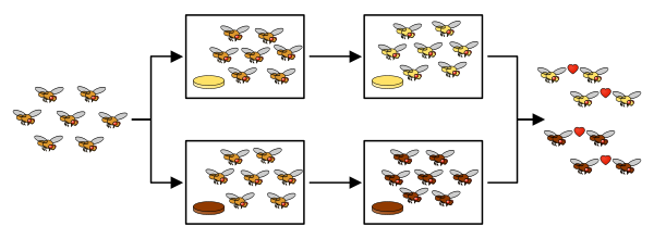
In simple terms, this is based on the idea that if gene flow has occurred across populations, then some alleles will have been transferred from one population to another. Because of this, we would expect that transferred alleles coalesce with alleles of the source population more recently than the divergence time of the two populations. Thus, models that include a migration rate often add it as a parameter specifying the probability than any given allele coalesces with an allele in another population or species (the backwards version of a migration or introgression event). Again, this might be difficult to conceptualise so there’s a handy diagram below.

Migration rate test figure — A similar model of coalescence as above, but testing for migration rate (gene flow) in two recently diverged populations (right). In this example, when we trace two alleles (red and green) back in time, we notice that some individuals in Population 1 coalesce more recently with individuals of Population 2 than other individuals of Population 1 (e.g. for the red allele), and vice versa for the green allele. This can also be represented with gene trees (left), with dashed lines representing individuals from Population 2 and whole lines representing individuals from Population 1. This incomplete split between the two populations is the result of migration transferring genes from one population to the other after their initial divergence (also called ‘introgression’ or ‘horizontal gene transfer’).

Testing divergence time

In a similar vein, the coalescent can also be used to test how long ago the two contemporary populations diverged. Similar to gene flow, this is often included as an additional parameter on top of the coalescent model in terms of the number of generations ago. To convert this to a meaningful time estimate (e.g. in terms of thousands or millions of years ago), we need to include a mutation rate (the number of mutations per base pair of sequence per generation) and a generation time for the study species (how many years apart different generations are: for humans, we would typically say ~20-30 years).

Divergence time test figure.jpg — An example of using the coalescent to test the divergence time between two populations, this time using three different alleles (red, green and yellow). Tracing back the coalescence of each alleles reveals different times (in terms of which generation the coalescence occurs in) depending on the allele (right). As above, we can look at this through gene trees (left), showing variation how far back the two populations (again indicated with bold and dashed lines respectively) split. The blue box indicates the range of times (i.e. a confidence interval) around which divergence occurred: with many more alleles, this can be more refined by using an ‘average’ and later related to time in years with a generation time.

The basic model of testing divergence time with the coalescent is relatively simple, and not all that different to phylogenetic methods. Where in phylogenetics we relate the length of the different branches in the tree to the amount of time that has occurred since the divergence of those branches, with the coalescent we base these on coalescent events, with more coalescent events occurring around the time of divergence. One important difference in the two methods is that coalescent events might not directly coincide with divergence time (in fact, we expect many do not) as some alleles will separate prior to divergence, and some will lag behind and start to diverge after the divergence event.

The complex nature of the coalescent

While each of these individual concepts may seem (depending on how well you handle maths!) relatively simple, one critical issue is the interactive nature of the different factors. Gene flow, divergence time and population size changes will all simultaneously impact the distribution and frequency of alleles and thus the coalescent method. Because of this, we often use complex programs to employ the coalescent which tests and balances the relative contributions of each of these factors to some extent. Although the coalescent is a complex beast, improvements in the methodology and the programs that use it will continue to improve our ability to infer evolutionary history with coalescent theory.

The space for species: how spatial aspects influence speciation

November 1, 2018November 1, 2018Sean Buckley2 Comments

Spatial and temporal factors of speciation

The processes driving genetic differentiation, and the progressive development of populations along the speciation continuum, are complex in nature and influenced by a number of factors. Generally, on The G-CAT we have considered the temporal aspects of these factors: how time much time is needed for genetic differentiation, how this might not be consistent across different populations or taxa, and how a history of environmental changes affect the evolution of populations and species. We’ve also touched on the spatial aspects of speciation and genetic differentiation before, but in significantly less detail.

To expand on this, we’re going to look at a few different models of how the spatial distribution of populations influences their divergence, and particularly how these factor into different processes of speciation.

What comes first, ecological or genetic divergence?

One key paradigm in understanding speciation is somewhat an analogy to the “chicken and the egg scenario”, albeit with ecological vs. genetic divergence. This concept is based on the idea that two aspects are key for determining the formation of new species: genetic differentiation of the populations in question, and ecological (or adaptive) changes that provide new ecological niches for species to inhabit. Without both, we might have new morphotypes or ecotypes of a singular species (in the case of ecological divergence without strong genetic divergence) or cryptic species (genetically distinct but ecologically identical species).

The order of these two processes have been in debate for some time, and different aspects of species and the environment can influence how (or if) these processes occur.

Different spatial models of speciation

Generally, when we consider the spatial models for speciation we divide these into distinct categories based on the physical distance of populations from one another. Although there is naturally a lot of grey area (as there is with almost everything in biological science), these broad concepts help us to define and determine how speciation is occurring in the wild.

Allopatric speciation

The simplest model is one we have described before called “allopatry”. In allopatry, populations are distributed distantly from one another, so that there are separated and isolated. A common way to imagine this is islands of populations separated by ocean of unsuitable habitat.

Allopatric speciation is considered one of the simplest and oldest models of speciation as the process is relatively straightforward. Geographic isolation of populations separates them from one another, meaning that gene flow is completely stopped and each population can evolve independently. Small changes in the genes of each population over time (e.g. due to different natural selection pressures) cause these populations to gradually diverge: eventually, this divergence will reach a point where the two populations would not be compatible (i.e. are reproductively isolated) and thus considered separate species.

Allopatry_example — The standard model of allopatric speciation, following an island model. 1) We start with a single population occupying a single island. 2) A rare dispersal event pushes some individuals onto a new island, forming a second population. Note that this doesn’t happen often enough to allow for consistent gene flow (i.e. the island was only colonised once). 3) Over time, these populations may accumulate independent genetic and ecological changes due to both natural selection and drift, and when they become so different that they are reproductively isolated they can be considered separate species.

Although relatively straightforward, one complex issue of allopatric speciation is providing evidence that hybridisation couldn’t happen if they reconnected, or if populations could be considered separate species if they could hybridise, but only under forced conditions (i.e. it is highly unlikely that the two ‘species’ would interact outside of experimental conditions).

Parapatric and peripatric speciation

A step closer in bringing populations geographically together in speciation is “parapatry” and “peripatry”. Parapatric populations are often geographically close together but not overlapping: generally, the edges of their distributions are touching but do not overlap one another. A good analogy would be to think of countries that share a common border. Parapatry can occur when a species is distributed across a broad area, but some form of narrow barrier cleaves the distribution in two: this can be the case across particular environmental gradients where two extremes are preferred over the middle.

The main difference between paraptry and allopatry is the allowance of a ‘hybrid zone’. This is the region between the two populations which may not be a complete isolating barrier (unlike the space between allopatric populations). The strength of the barrier (and thus the amount of hybridisation and gene flow across the two populations) is often determined by the strength of the selective pressure (e.g. how unfit hybrids are). Paraptry is expected to reduce the rate and likelihood of speciation occurring as some (even if reduced) gene flow across populations is reduces the amount of genetic differentiation between those populations: however, speciation can still occur.

Parapatric speciation across a thermocline.jpg — An example of parapatric species across an environment gradient (in this case, a temperature gradient along the ocean coastline). **Left:** We have two main species (red and green fish) which are adapted to either hotter or colder temperatures (red and green in the gradient), respectively. A small zone of overlap exists where hybrid fish (yellow) occur due to intermediate temperature. **Right:** How the temperature varies across the system, forming a steep gradient between hot and cold waters.

Related to this are peripatric populations. This differs from parapatry only slightly in that one population is an original ‘source’ population and the other is a ‘peripheral’ population. This can happen from a new population becoming founded from the source by a rare dispersal event, generating a new (but isolated) population which may diverge independently of the source. Alternatively, peripatric populations can be formed when the broad, original distribution of the species is reduced during a population contraction, and a remnant piece of the distribution becomes fragmented and ‘left behind’ in the process, isolated from the main body. Speciation can occur following similar processes of allopatric speciation if gene flow is entirely interrupted or paraptric if it is significantly reduced but still present.

Peripatric distributions.jpg — The two main ways peripatric species can form. **Left:** The dispersal method. In this example, there is a central ‘source’ population (orange birds on the main island), which holds most of the distribution. However, occasionally (more frequently than in the allopatric example above) birds can disperse over to the smaller island, forming a (mostly) independent secondary population. If the gene flow between this population and the central population doesn’t overwhelm the divergence between the two populations (due to selection and drift), then a new species (blue birds) can form despite the gene flow. **Right:** The range contraction method. In this example, we start with a single widespread population (blue lizards) which has a rapid reduction in its range. However, during this contraction one population is separated from the main body (i.e. as a refugia), which may also be a precursor of peripatric speciation.

Sympatric (ecological) speciation

On the other end of the distribution spectrum, the two diverging populations undergoing speciation may actually have completely overlapping distributions. In this case, we refer to these populations as “sympatric”, and the possibility of sympatric speciation has been a highly debated topic in evolutionary biology for some time. One central argument rears its head against the possibility of sympatric speciation, in that if populations are co-occurring but not yet independent species, then gene flow should (theoretically) occur across the populations and prevent divergence.

It is in sympatric speciation that we see the opposite order of ecological and genetic divergence happen. Because of this, the process is often referred to as “ecological speciation”, where individual populations adapt to different niches within the same area, isolating themselves from one another by limiting their occurrence and tolerances. As the two populations are restricted from one another by some kind of ecological constraint, they genetically diverge over time and speciation can occur.

This can be tricky to visualise, so let’s invent an example. Say we have a tropical island, which is occupied by one bird species. This bird prefers to eat the large native fruit of the island, although there is another fruit tree which produces smaller fruits. However, there’s only so much space and eventually there are too many birds for the number of large fruit trees available. So, some birds are pushed to eat the smaller fruit, and adapt to a different diet, changing physiology over time to better acquire their new food and obtain nutrients. This shift in ecological niche causes the two populations to become genetically separated as small-fruit-eating-birds interact more with other small-fruit-eating-birds than large-fruit-eating-birds. Over time, these divergences in genetics and ecology causes the two populations to form reproductively isolated species despite occupying the same island.

Ecological sympatric speciation — A diagram of the ecological speciation example given above. Note that ecological divergence occurs first, with some birds of the original species shifting to the new food source (‘ecological niche’) which then leads to speciation. An important requirement for this is that gene flow is somehow (even if not totally) impeded by the ecological divergence: this could be due to birds preferring to mate exclusively with other birds that share the same food type; different breeding seasons associated with food resources; or other isolating mechanisms.

Although this might sound like a simplified example (and it is, no doubt) of sympatric speciation, it’s a basic summary of how we ended up with so many species of Darwin’s finches (and why they are a great model for the process of evolution by natural selection).

The complexity of speciation

As you can see, the processes and context driving speciation are complex to unravel and many factors play a role in the transition from population to species. Understanding the factors that drive the formation of new species is critical to understanding not just how evolution works, but also in how new diversity is generated and maintained across the globe (and how that might change in the future).

What’s the (allele) frequency, Kenneth?

October 24, 2018October 24, 2018Sean Buckley5 Comments

Allele frequency

A number of times before on The G-CAT, we’ve discussed the idea of using the frequency of different genetic variants (alleles) within a particular population or species to test a number of different questions about evolution, ecology and conservation. These are all based on the central notion that certain forces of nature will alter the distribution and frequency of alleles within and across populations, and that these patterns are somewhat predictable in how they change.

One particular distinction we need to make early here is the difference between allele frequency and allele identity. In these analyses, often we are working with the same alleles (i.e. particular variants) across our populations, it’s just that each of these populations may possess these particular alleles in different frequencies. For example, one population may have an allele (let’s call it Allele A) very rarely – maybe only 10% of individuals in that population possess it – but in another population it’s very common and perhaps 80% of individuals have it. This is a different level of differentiation than comparing how different alleles mutate (as in the coalescent) or how these mutations accumulate over time (like in many phylogenetic-based analyses).

Allele freq vs identity figure.jpg — An example of the difference between allele frequency and identity. In this example (and many of the figures that follow in this post), the circle denote different populations, within which there are individuals which possess either an A gene (blue) or a B gene. **Left:** If we compared Populations 1 and 2, we can see that they both have A and B alleles. However, these alleles vary in their frequency within each population, with an equal balance of A and B in Pop 1 and a much higher frequency of B in Pop 2. **Right:** However, when we compared Pop 3 and 4, we can see that not only do they vary in frequencies, they vary in the presence of alleles, with one allele in each population but not the other.

Non-adaptive (neutral) uses

Testing neutral structure

Arguably one of the most standard uses of allele frequency data is the determination of population structure, one which more avid The G-CAT readers will be familiar with. This is based on the idea that populations that are isolated from one another are less likely to share alleles (and thus have similar frequencies of those alleles) than populations that are connected. This is because gene flow across two populations helps to homogenise the frequency of alleles within those populations, by either diluting common alleles or spreading rarer ones (in general). There are a number of programs that use allele frequency data to assess population structure, but one of the most common ones is STRUCTURE.

Gene flow homogeneity figure — An example of how gene flow across populations homogenises allele frequencies. We start with two initial populations (1 and 2 from above), which have very different allele frequencies. Hybridising individuals across the two populations means some alleles move from Pop 1 and Pop 2 into the hybrid population: which alleles moves is random (the smaller circles). Because of this, the resultant hybrid population has an allele frequency somewhere in between the two source populations: think of like mixing red and blue cordial and getting a purple drink.

Simple YPP structure figure.jpg — An example of a Structure plot which long-term *The G-CAT* readers may be familiar with. This is taken from Brauer *et al.* (2013), where the authors studied the population structure of the Yarra pygmy perch. Each small column represents a single individual, with the colours representing how well the alleles of that individual fit a particular genetic population (each population has one colour). The numbers and broader columns refer to different ‘localities’ (different from populations) where individuals were sourced. This shows clear strong population structure across the 4 main groups, except for in Locality 6 where there is a mixture of Eastern and Merri/Curdies alleles.

Determining genetic bottlenecks and demographic change

Other neutral aspects of population identity and history can be studied using allele frequency data. One big component of understanding population history in particular is determining how the population size has changed over time, and relating this to bottleneck events or expansion periods. Although there are a number of different approaches to this, which span many types of analyses (e.g. also coalescent methods), allele frequency data is particularly suited to determining changes in the recent past (hundreds of generations, as opposed to thousands of generations ago). This is because we expect that, during a bottleneck event, it is statistically more likely for rare alleles (i.e. those with low frequency) in the population to be lost due to strong genetic drift: because of this, the population coming out of the bottleneck event should have an excess of more frequent alleles compared to a non-bottlenecked population. We can determine if this is the case with tests such as the heterozygosity excess, M-ratio or mode shift tests.

Genetic drift and allele freq figure — A diagram of how allele frequencies change in genetic bottlenecks due to genetic drift. **Left:** Large circles again denote a population (although across different sequential times), with smaller circle denoting which alleles survive into the next generation (indicated by the coloured arrows). We start with an initial ‘large’ population of 8, which is reduced down to 4 and 2 in respective future times. Each time the population contracts, only a select number of alleles (or individuals) ‘survive’: assuming no natural selection is in process, this is totally random from the available gene pool. **Right:** We can see that over time, the frequencies of alleles A and B shift dramatically, leading to the ‘extinction’ of Allele B due to genetic drift. This is because it is the less frequent allele of the two, and in the smaller population size has much less chance of randomly ‘surviving’ the purge of the genetic bottleneck.

Adaptive (selective) uses

Testing different types of selection

We’ve also discussed previously about how different types of natural selection can alter the distribution of allele frequency within a population. There are a number of different predictions we can make based on the selective force and the overall population. For understanding particular alleles that are under strong selective pressure (i.e. are either strongly adaptive or maladaptive), we often test for alleles which have a frequency that strongly deviates from the ‘neutral’ background pattern of the population. These are called ‘outlier loci’, and the fact that their frequency is much more different from the average across the genome is attributed to natural selection placing strong pressure on either maintaining or removing that allele.

Other selective tests are based on the idea of correlating the frequency of alleles with a particular selective environmental pressure, such as temperature or precipitation. In this case, we expect that alleles under selection will vary in relation to the environmental variable. For example, if a particular allele confers a selective benefit under hotter temperatures, we would expect that allele to be more common in populations that occur in hotter climates and rarer in populations that occur in colder climates. This is referred to as a ‘genotype-environment association test’ and is a good way to detect polymorphic selection (i.e. when multiple alleles contribute to a change in a single phenotypic trait).

Genotype by environment figure.jpg — An example of how the frequency of alleles might vary under natural selection in correlation to the environment. In this example, the blue allele A is adaptive and under positive selection in the more intense environment, and thus increases in frequency at higher values. Contrastingly, the red allele B is maladaptive in these environments and decreases in frequency. For comparison, the black allele shows how the frequency of a neutral (non-adaptive or maladaptive) allele doesn’t vary with the environment, as it plays no role in natural selection.

Taxonomic (species identity) uses

At one end of the spectrum of allele frequencies, we can also test for what we call ‘fixed differences’ between populations. An allele is considered ‘fixed’ it is the only allele for that locus in the population (i.e. has a frequency of 1), whilst the alternative allele (which may exist in other populations) has a frequency of 0. Expanding on this, ‘fixed differences’ occur when one population has Allele A fixed and another population has Allele B fixed: thus, the two populations have as different allele frequencies (for that one locus, anyway) as possible.

Fixed differences are sometimes used as a type of diagnostic trait for species. This means that each ‘species’ has genetic variants that are not shared at all with its closest relative species, and that these variants are so strongly under selection that there is no diversity at those loci. Often, fixed differences are considered a level above populations that differ by allelic frequency only as these alleles are considered ‘diagnostic’ for each species.

Fixed differences figure.jpg — An example of the difference between fixed differences and allelic frequency differences. In this example, we have 5 cats from 3 different species, sequencing a particular target gene. Within this gene, there are three possible alleles: **T, A** or G respectively. You’ll quickly notice that the T allele is both unique to Species A and is present in all cats of that species (i.e. is fixed). This is a fixed difference between Species A and the other two. Alleles A and G, however, are present in both Species B and C, and thus are not fixed differences even if they have different frequencies.

Intrapopulation (relatedness) uses

Allele frequency-based methods are even used in determining relatedness between individuals. While it might seem intuitive to just check whether individuals share the same alleles (and are thus related), it can be hard to distinguish between whether they are genetically similar due to direct inheritance or whether the entire population is just ‘naturally’ similar, especially at a particular locus. This is the distinction between ‘identical-by-descent’, where alleles that are similar across individuals have recently been inherited from a similar ancestor (e.g. a parent or grandparent) or ‘identical-by-state’, where alleles are similar just by chance. The latter doesn’t contribute or determine relatedness as all individuals (whether they are directly related or not) within a population may be similar.

To distinguish between the two, we often use the overall frequency of alleles in a population as a basis for determining how likely two individuals share an allele by random chance. If alleles which are relatively rare in the overall population are shared by two individuals, we expect that this similarity is due to family structure rather than population history. By factoring this into our relatedness estimates we can get a more accurate overview of how likely two individuals are to be related using genetic information.

The wild world of allele frequency

Despite appearances, this is just a brief foray into the many applications of allele frequency data in evolution, ecology and conservation studies. There are a plethora of different programs and methods that can utilise this information to address a variety of scientific questions and refine our investigations.

Short essay: Real life or (‘just’) fantasy?

October 18, 2018Sean Buckley1 Comment

The fantastical

Like many people, from a young age I was obsessed and interested in works of fantasy and science fiction. To feel transported to magical worlds of various imaginative creatures and diverse places. The luxury of being able to separate from the mundanity of reality is one many children (or nostalgic adults) will be able to relate to upon reflection. Worlds that appear far more creative and engaging than our own are intrinsically enticing to the human psyche and the escapism it allows is no doubt an integral part of growing up for many people (especially those who have also dealt or avoided dealing with mental health issues).

The biological

The intricate connection to the (super)natural world drove me to fall in love with the natural world. Although there might seem to be an intrinsic contrast between the two – the absence or presence of reality – the truth is that the world is a wondrous place if you observe it through an appropriate lens. Dragons are real, forms of life are astronomically varied and imaginative, and there we are surrounded by the unknown and potentially mythical. To see the awe and mystification on a child’s face when they see a strange or unique animal for the very first time bears remarkable parallels to the expression when we stare into the fantasy of Avatar or The Lord of the Rings.

Combined dragon images — Two (very different) types of real life dragons. On the left, a terrifying dragon fish brought up from the abyssal depths by the CSIRO *RV Investigator* expedition. On the right, the minuscule but beautiful blue dragon (*Glaucus atlanticus*), which is actually a slug.

It might seem common for ‘nerds’ (at least under the traditional definition of being obsessed with particular aspects of pop culture) to later become scientists of some form or another. And I think this is a true reflection: particularly, I think the innate personality traits that cause one to look at the world of fantasy with wonder and amazement also commonly elicits a similar response in terms of the natural world. It is hard to see an example where the CGI’d majesty of contemporary fantasy and sci-fi could outcompete the intrigue generated by real, wondrous plants and animals.

Seeing the divine in the mundane

Although we often require a more tangible, objective justification for research, the connection of people to the diversity of life (whether said diversity is fictitious or not) should be a significant driving factor in the perceived importance of conservation management. However, we are often degraded to somewhat trivial discussions: why should we care about (x) species? What do they do for us? Why are they important?

Combined baobab images — Sometimes the ‘mundane’ (real) can inspire the ‘fantasy’… On the left, a real baobab tree (genus *Adansonia*: this one is *Adansonia grandidieri*) from Madagascar. On the right, the destructive baobab trees threaten to tear apart the prince’s planet in ‘*The Little Prince’* by Antoine de Saint-Exupéry.

If we approach the real world and the organisms that inhabit it with truly the same wonder as we approach the fantastical, would we be more successful in preserving biodiversity? Could we reverse our horrific trend of letting species go extinct? Every species on Earth represents something unique: a new perspective, an evolutionary innovation, a lens through which to see the world and its history. Even the most ‘mundane’ of species represent something critical to functionality of ecosystems, and their lack of emphasis undermines their importance.

Dementor wasp.png — …and sometimes, the fantasy inspires the reality. This is the dementor wasp (*Ampulex dementor*), named after the frightening creatures from the ‘*Harry Potter*‘ series. The name was chosen by the public based on the behaviour of the wasp to inject a toxin into its cockroach prey, which effectively turns them into mindless zombies and makes them unable to resist being pulled helplessly into the wasp’s nest. Absolutely terrifying.

The biota of Earth are no different to the magical fabled beasts of science fiction and fantasy, and we’re watching it all burn away right in front of our eyes.

You’re perfect, you’re beautiful, you look like a model (species)

October 11, 2018Sean Buckley1 Comment

What is a ‘model’?

There are quite literally millions of species on Earth, ranging from the smallest of microbes to the largest of mammals. In fact, there are so many that we don’t actually have a good count on the sheer number of species and can only estimate it based on the species we actually know about. Unsurprisingly, then, the number of species vastly outweighs the number of people that research them, especially considering the sheer volumes of different aspects of species, evolution, conservation and their changes we could possibly study.

Species on Earth estimate figure — Some estimations on the number of eukaryotic species (i.e. not including things like bacteria), with the number of known species in blue and the predicted number of total species on Earth in purple. Source: Census of Marine Life.

This is partly where the concept of a ‘model’ comes into it: it’s much easier to pick a particular species to study as a target, and use the information from it to apply to other scenarios. Most people would be familiar with the concept based on medical research: the ‘lab rat’ (or mouse). The common house mouse (Mus musculus) and the brown rat (Rattus norvegicus) are some of the most widely used models for understanding the impact of particular biochemical compounds on physiology and are often used as the testing phase of medical developments before human trials.

So, why are mice used as a ‘model’? What actually constitutes a ‘model’, rather than just a ‘relatively-well-research-species’? Well, there are a number of traits that might make certain species ideal subjects for understanding key concepts in evolution, biology, medicine and ecology. For example, mice are often used in medical research given their (relative) similar genetic, physiological and behavioural characteristics to humans. They’re also relatively short-lived and readily breed, making them ideal to observe the more long-term effects of medical drugs or intergenerational impacts. Other species used as models primarily in medicine include nematodes (Caenorhabditis elegans), pigs (Sus scrofa domesticus), and guinea pigs (Cavia porcellus).

The diversity of models

There are a wide variety and number of different model species, based on the type of research most relevant to them (and how well it can be applied to other species). Even with evolution and conservation-based research, which can often focus on more obscure or cryptic species, there are several key species that have widely been applied as models for our understanding of the evolutionary process. Let’s take a look at a few examples for evolution and conservation.

Drosophila

It would be remiss of me to not mention one of the most significant contributors to our understanding of the genetic underpinning of adaptation and speciation, the humble fruit fly (Drosophila melanogaster, among other species). The ability to rapidly produce new generations (with large numbers of offspring with very short generation time), small fully-sequenced genome, and physiological variation means that observing both phenotypic and genotypic changes over generations due to ‘natural’ (or ‘experimental’) selection are possible. In fact, Drosphilia spp. were key in demonstrating the formation of a new species under laboratory conditions, providing empirical evidence for the process of natural selection leading to speciation (despite some creationist claims that this has never happened).

Darwin’s finches

The original model of evolution could be argued to be Darwin’s finches, as the formed part of the empirical basis of Charles Darwin’s work on the theory of evolution by natural selection. This is because the different species demonstrate very distinct and obvious changes in morphology related to a particular diet (e.g. the physiological consequences of natural selection), spread across an archipelago in a clear demonstration of a natural experiment. Thus, they remain the original example of adaptive radiation and are fundamental components of the theory of evolution by natural selection. However, surprisingly, Darwin’s finches are somewhat overshadowed in modern research by other species in terms of the amount of available data.

Zebra finches

Even as far as birds go, one species clearly outshines the rest in terms of research. The zebra finch is one of the most highly researched vertebrate species, particularly as a model of song learning and behaviour in birds but also as a genetic model. The full genome of the zebra finch was the second bird to ever be sequenced (the first being a chicken), and remains one of the more detailed and annotated genomes in birds. Because of this, the zebra finch genome is often used as a reference for other studies on the genetics of bird species, especially when trying to understand the function of genetic changes or genes under selection.

Fishes

Fish are (perhaps surprisingly) also relatively well research in terms of evolutionary studies, largely due to their ancient origins and highly diverse nature, with many different species across the globe. They also often demonstrate very rapid and strong bouts of divergence, such as the cichlid fish species of African lakes which demonstrate how new species can rapidly form when introduced to new and variable environments. The cichlids have become the poster child of adaptive radiation in fishes much in the same way that Darwin’s finches highlighted this trend in birds. Another group of fish species used as a model for similar aspects of speciation, adaptive divergence and rapid evolutionary change are the three-spine and nine-spine stickleback species, which inhabit a variety of marine, estuarine and freshwater environments. Thus, studies on the genetic changes across these different morphotypes is a key in understanding how adaptation to new environments occur in nature (particularly the relatively common transition into different water types in fishes).

cichlid diversity figure — The sheer diversity of species and form makes African cichlids an ideal model for testing hypotheses and theories about the process of evolution and adaptive radiation. Figure sourced from Brawand *et al.* (2014) in Nature.

Zebra fish

More similar to the medical context of lab rats is the zebrafish (ironically, zebra themselves are not considered a model species). Zebrafish are often used as models for understanding embryology and the development of the body in early formation given the rapid speed at which embryonic development occurs and the transparent body of embryos (which makes it easier to detect morphological changes during embryogenesis).

Using information from model species for non-models

While the relevance of information collected from model species to other non-model species depends on the similarity in traits of the two species, our understanding of broad concepts such as evolutionary process, biochemical pathways and physiological developments have significantly improved due to model species. Applying theories and concepts from better understood organisms to less researched ones allows us to produce better research much faster by cutting out some of the initial investigative work on the underlying processes. Thus, model species remain fundamental to medical advancement and evolutionary theory.

That said, in an ideal world all species would have the same level of research and resources as our model species. In this sense, we must continue to strive to understand and research the diversity of life on Earth, to better understand the world in which we live. Full genomes are progressively being sequenced for more and more species, and there are a number of excellent projects that are aiming to sequence at least one genome for all species of different taxonomic groups (e.g. birds, bats, fish). As the data improves for our non-model species, our understanding of evolution, conservation management and medical research will similarly improve.