The reality of neutrality

The neutral theory

Many, many times within The G-CAT we’ve discussed the difference between neutral and selective processes, DNA markers and their applications in our studies of evolution, conservation and ecology. The idea that many parts of the genome evolve under a seemingly random pattern – largely dictated by genome-wide genetic drift rather than the specific force of natural selection – underpins many demographic and adaptive (in outlier tests) analyses.

This is based on the idea that for genes that are not related to traits under selection (either positively or negatively), new mutations should be acquired and lost under predominantly random patterns. Although this accumulation of mutations is influenced to some degree by alternate factors such as population size, the overall average of a genome should give a picture that largely discounts natural selection. But is this true? Is the genome truly neutral if averaged?

Non-neutrality

First, let’s take a look at what we mean by neutral or not. For genes that are not under selection, alleles should be maintained at approximately balanced frequencies and all non-adaptive genes across the genome should have relatively similar distribution of frequencies. While natural selection is one obvious way allele frequencies can be altered (either favourably or detrimentally), other factors can play a role.

As stated above, population sizes have a strong impact on allele frequencies. This is because smaller populations are more at risk of losing rarer alleles due to random deaths (see previous posts for a more thorough discussion of this). Additionally, genes which are physically close to other genes which are under selection may themselves appear to be under selection due to linkage disequilibrium (often shortened to ‘LD’). This is because physically close genes are more likely to be inherited together, thus selective genes can ‘pull’ neighbours with them to alter their allele frequencies.

Linkage disequilibrium figure — An example of how linkage disequilibrium can alter allele frequency of ‘neutral’ parts of the genome as well. In this example, only one part of this section of the genome is selected for: the **green gene**. Because of this positive selection, the frequency of a particular allele at this gene increases (the **blue graph**): however, nearby parts of the genome also increase in frequency due to their proximity to this selected gene, which decreases with distance. The extent of this effect determines the size of the ‘linkage block’ (see below).

Why might ‘neutral’ models not be neutral?

The assumption that the vast majority of the genome evolves under neutral patterns has long underpinned many concepts of population and evolutionary genetics. But it’s never been all that clear exactly how much of the genome is actually evolving neutrally or adaptively. How far natural selection reaches beyond a single gene under selection depends on a few different factors: let’s take a look at a few of them.

Linked selection

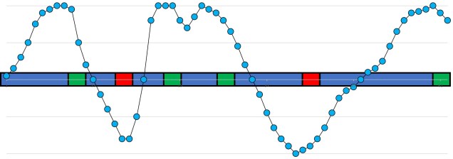
As described above, physically close genes (i.e. located near one another on a chromosome) often share some impacts of selection due to reduced recombination that occurs at that part of the genome. In this case, even alleles that are not adaptive (or maladaptive) may have altered frequencies simply due to their proximity to a gene that is under selection (either positive or negative).

Recombination blocks and linkage figure — A (perhaps familiar) example of the interaction between recombination (the breaking and mixing of different genes across chromosomes) and linkage disequilibrium. In this example, we have 5 different copies of a part of the genome (**different coloured sequences**), which we randomly ‘break’ into separate fragments (**breaks indicated by the dashed lines**). If we focus on a particular base in the sequence (the **yellow A**) and count the number of times a particular base pair is on the same fragment, we can see how physically close bases are more likely to be coinherited than further ones (**bottom column graph**). This makes mathematical sense: if two bases are further apart, you’re more likely to have a break that separates them. This is the very basic underpinning of linkage and recombination, and the size of the region where bases are likely to be coinherited is called the ‘linkage block’.

Under these circumstances, for a region of a certain distance (dubbed the ‘linkage block’) around a gene under selection, the genome will not truly evolve neutrally. Although this is simplest to visualise as physically linked sections of the genome (i.e. adjacent), linked genes do not necessarily have to be next to one another, just linked somehow. For example, they may be different parts of a single protein pathway.

The extent of this linkage effect depends on a number of other factors such as ploidy (the number of copies of a chromosome a species has), the size of the population and the strength of selection around the central locus. The presence of linkage and its impact on the distribution of genetic diversity (LD) has been well documented within evolutionary and ecological genetic literature. The more pressing question is one of extent: how much of the genome has been impacted by linkage? Is any of the genome unaffected by the process?

Background selection

One example of linked selection commonly used to explain the proliferation of non-neutral evolution within the genome is ‘background selection’. Put simply, background selection is the purging of alleles due to negative selection on a linked gene. Sometimes, background selection is expanded to include any forms of linked selection.

Under the first etymology of background selection, the process can be divided into two categories based on the impact of the linkage. As above, one scenario is the purging of neutral alleles (and therefore reduction in genetic diversity) as it is associated with a deleterious maladaptive gene nearby. Contrastingly, some neutral alleles may be preserved by association with a positively selected adaptive gene: this is often referred to as ‘genetic hitchhiking’ (which I’ve always thought was kind of an amusing phrase…).

Genetic hitchhiking picture.jpg — Definitely not how genetic hitchhiking works.

The presence of background selection – particularly under the ‘maladaptive’ scenario – is often used as a counter-argument to the ‘paradox in variation’. This paradox was determined by evolutionary biologist Richard Lewontin, who noted that despite massive differences in population sizes across the many different species on Earth, the total amount of ‘neutral’ genetic variation does not change significantly. In fact, he observed no clear relationship (directly) between population size and neutral variation. Many years after this observation, the influence of background selection and genetic hitchhiking on the distribution of genomic diversity helps to explain how the amount of neutral genomic variation is ‘managed’, and why it doesn’t vary excessively across biota.

What does it mean if neutrality is dead?

This findings have significant implications for our understanding of the process of evolution, and how we can detect adaptation within the genome. In light of this research, there has been heated discussion about whether or not neutral theory is ‘dead’, or a useful concept.

Genome wide allele frequency figure.jpg — A vague summary of how a large portion of the genome might not actually be neutral. In this section of the genome, we have neutral (**blue**), maladaptive (**red**) and adaptive (**green**) elements. Natural selection either favours, disfavours, or is ambivalent about each of this sections alone. However, there is significant ‘spill-over’ around regions of positively or negatively selected sections, which causes the allele frequency of even the neutral sections to fluctuate widely. The **blue dotted line** represents this: when the line is above the genome, allele frequency is increased; when it is below it is decreased. As we travel along this section of the genome, you may notice it is rarely ever in the middle (the so-called ‘neutral‘ allele frequency, in line with the genome).

Although I avoid having a strong stance here (if you’re an evolutionary geneticist yourself, I will allow you to draw your own conclusions), it is my belief that the model of neutral theory – and the methods that rely upon it – are still fundamental to our understanding of evolution. Although it may present itself as a more conservative way to identify adaptation within the genome, and cannot account for the effect of the above processes, neutral theory undoubtedly presents itself as a direct and well-implemented strategy to understand adaptation and demography.