Adaptation

You’re perfect, you’re beautiful, you look like a model (species)

October 11, 2018Sean Buckley1 Comment

What is a ‘model’?

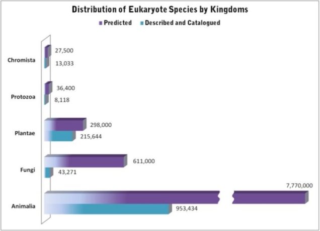
There are quite literally millions of species on Earth, ranging from the smallest of microbes to the largest of mammals. In fact, there are so many that we don’t actually have a good count on the sheer number of species and can only estimate it based on the species we actually know about. Unsurprisingly, then, the number of species vastly outweighs the number of people that research them, especially considering the sheer volumes of different aspects of species, evolution, conservation and their changes we could possibly study.

Species on Earth estimate figure — Some estimations on the number of eukaryotic species (i.e. not including things like bacteria), with the number of known species in blue and the predicted number of total species on Earth in purple. Source: Census of Marine Life.

This is partly where the concept of a ‘model’ comes into it: it’s much easier to pick a particular species to study as a target, and use the information from it to apply to other scenarios. Most people would be familiar with the concept based on medical research: the ‘lab rat’ (or mouse). The common house mouse (Mus musculus) and the brown rat (Rattus norvegicus) are some of the most widely used models for understanding the impact of particular biochemical compounds on physiology and are often used as the testing phase of medical developments before human trials.

So, why are mice used as a ‘model’? What actually constitutes a ‘model’, rather than just a ‘relatively-well-research-species’? Well, there are a number of traits that might make certain species ideal subjects for understanding key concepts in evolution, biology, medicine and ecology. For example, mice are often used in medical research given their (relative) similar genetic, physiological and behavioural characteristics to humans. They’re also relatively short-lived and readily breed, making them ideal to observe the more long-term effects of medical drugs or intergenerational impacts. Other species used as models primarily in medicine include nematodes (Caenorhabditis elegans), pigs (Sus scrofa domesticus), and guinea pigs (Cavia porcellus).

The diversity of models

There are a wide variety and number of different model species, based on the type of research most relevant to them (and how well it can be applied to other species). Even with evolution and conservation-based research, which can often focus on more obscure or cryptic species, there are several key species that have widely been applied as models for our understanding of the evolutionary process. Let’s take a look at a few examples for evolution and conservation.

Drosophila

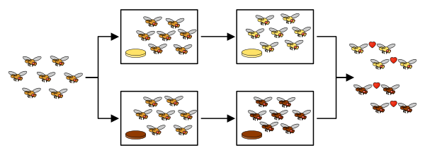
It would be remiss of me to not mention one of the most significant contributors to our understanding of the genetic underpinning of adaptation and speciation, the humble fruit fly (Drosophila melanogaster, among other species). The ability to rapidly produce new generations (with large numbers of offspring with very short generation time), small fully-sequenced genome, and physiological variation means that observing both phenotypic and genotypic changes over generations due to ‘natural’ (or ‘experimental’) selection are possible. In fact, Drosphilia spp. were key in demonstrating the formation of a new species under laboratory conditions, providing empirical evidence for the process of natural selection leading to speciation (despite some creationist claims that this has never happened).

Darwin’s finches

The original model of evolution could be argued to be Darwin’s finches, as the formed part of the empirical basis of Charles Darwin’s work on the theory of evolution by natural selection. This is because the different species demonstrate very distinct and obvious changes in morphology related to a particular diet (e.g. the physiological consequences of natural selection), spread across an archipelago in a clear demonstration of a natural experiment. Thus, they remain the original example of adaptive radiation and are fundamental components of the theory of evolution by natural selection. However, surprisingly, Darwin’s finches are somewhat overshadowed in modern research by other species in terms of the amount of available data.

Zebra finches

Even as far as birds go, one species clearly outshines the rest in terms of research. The zebra finch is one of the most highly researched vertebrate species, particularly as a model of song learning and behaviour in birds but also as a genetic model. The full genome of the zebra finch was the second bird to ever be sequenced (the first being a chicken), and remains one of the more detailed and annotated genomes in birds. Because of this, the zebra finch genome is often used as a reference for other studies on the genetics of bird species, especially when trying to understand the function of genetic changes or genes under selection.

Fishes

Fish are (perhaps surprisingly) also relatively well research in terms of evolutionary studies, largely due to their ancient origins and highly diverse nature, with many different species across the globe. They also often demonstrate very rapid and strong bouts of divergence, such as the cichlid fish species of African lakes which demonstrate how new species can rapidly form when introduced to new and variable environments. The cichlids have become the poster child of adaptive radiation in fishes much in the same way that Darwin’s finches highlighted this trend in birds. Another group of fish species used as a model for similar aspects of speciation, adaptive divergence and rapid evolutionary change are the three-spine and nine-spine stickleback species, which inhabit a variety of marine, estuarine and freshwater environments. Thus, studies on the genetic changes across these different morphotypes is a key in understanding how adaptation to new environments occur in nature (particularly the relatively common transition into different water types in fishes).

cichlid diversity figure — The sheer diversity of species and form makes African cichlids an ideal model for testing hypotheses and theories about the process of evolution and adaptive radiation. Figure sourced from Brawand *et al.* (2014) in Nature.

Zebra fish

More similar to the medical context of lab rats is the zebrafish (ironically, zebra themselves are not considered a model species). Zebrafish are often used as models for understanding embryology and the development of the body in early formation given the rapid speed at which embryonic development occurs and the transparent body of embryos (which makes it easier to detect morphological changes during embryogenesis).

Using information from model species for non-models

While the relevance of information collected from model species to other non-model species depends on the similarity in traits of the two species, our understanding of broad concepts such as evolutionary process, biochemical pathways and physiological developments have significantly improved due to model species. Applying theories and concepts from better understood organisms to less researched ones allows us to produce better research much faster by cutting out some of the initial investigative work on the underlying processes. Thus, model species remain fundamental to medical advancement and evolutionary theory.

That said, in an ideal world all species would have the same level of research and resources as our model species. In this sense, we must continue to strive to understand and research the diversity of life on Earth, to better understand the world in which we live. Full genomes are progressively being sequenced for more and more species, and there are a number of excellent projects that are aiming to sequence at least one genome for all species of different taxonomic groups (e.g. birds, bats, fish). As the data improves for our non-model species, our understanding of evolution, conservation management and medical research will similarly improve.

The MolEcol Toolbox: Species Distribution Modelling

September 12, 2018Sean Buckley4 Comments

Where on Earth are species?

Understanding the spatial distribution of species is a critical component for many different aspects of biological studies. Particularly for conservation, the biogeography of regions is a determinant factor for designating and managing biodiversity hotspots and management units. Or understanding the biogeographical mechanisms that have shaped modern biodiversity may allow us to understand how species will change under future climate change scenarios, and how their distributions will (and have) shift(ed).

Typically, the maximum distribution of species is based on their ecological tolerances: that is, the most extreme environments they can tolerate and proliferate within. Of course, there are a huge number of other factors on top of just natural environment which can shape species distributions, particularly related to human-induced environmental changes (or introducing new species as invasive pests, which we seem to be good at). But exactly where species are and why they occur there are intrinsically linked to the adaptive characteristics of species relative to their environment.

Species distribution modelling

The connection of a species distribution with innate environmental tolerances is the background for a type of analysis we call species distribution modelling (SDM) or environmental niche modelling (ENM). Species distribution modelling seeks to correlate the locations where a species occurs with the local environment around those sites to predict where the species should occur. This is an effective tool for trying to understand the distribution of species that might be tricky to study so thoroughly in the wild; either because they are hard to catch, live in very remote areas, or because they are highly threatened. There are a number of different algorithms and data types that will work with SDM, and there is always ongoing debate about ‘best practices’ in modelling techniques.

SDM method.jpg — The generalised pipeline of SDM, taken from Svenning *et al.* (2011). By correlating species occurrence data (bottom left) with environmental data (top left), we can develop a model that describes how the species is distributed based on environmental limitations (top right). From here, we can choose to validate the model with other methods (top and bottom centre) or see how the distribution might change with different environmental changes (e.g. bottom right).

A basic how-to on running SDM

The first major component that is needed for SDM is the occurrence data. Some methods will work with presence-only data: that is, a map of GPS coordinates which describes where that species has been found. Others work with presence-absence data, which may require including sites of known non-occurrence. This is an important aspect as the non-occurring sites defines the environment beyond the tolerance threshold of the species: however, it’s very likely that we haven’t sampled every location where they occur, and there will be some GPS co-ordinates that appear to be absent of our species where they actually occur. There are some different analytical techniques which can account for uneven sampling across the real distribution of the species, but they can get very technical.

An example of species (occurrence only) locality data (with >72,000 records) for the koala (*Phascolarctos cinereus*) across Australia, taken from the Atlas of Living Australia. Carefully checking the locality data is important, as visual inspection clearly shows records where koalas are not native: they might have been recorded from an introduced individual, given incorrect GPS coordinates or incorrectly identified (**red circles**).

The second major component is our environmental data. Typically, we want to include environmental data for the types of variables that are likely to constrain the distribution of our species: often temperature and precipitation variables are included, as these two largely predict habitat types. However, it can also be important to include non-climatic variables such as topography (e.g. elevation, slope) in our model to help constrain our predictions to a more reasonable area. It is also important to test for correlation between our variables, as using many variables which are highly correlated may ‘overfit’ the model and underestimate the range of the distribution by placing an unrealistic number of restrictions on the model.

An example of some of the environmental data/maps we might choose to include in a species distribution model, obtained from the Atlas of Living Australia. A) Mean annual temperature. B) Mean annual precipitation. C) Elevation. D) Weighted distance to nearest waterbody (e.g. rivers, lakes, streams).

Our SDM analysis of choice (e.g. MaxEnt) will then use various algorithms to build a model which best correlates where the species occurs with the environmental variables at those sites. The model tries to create a set of environmental conditions that best encapsulate the occurrence sites whilst excluding the non-occurrence sites from the prediction. From the final model, we can evaluate how strong the effect of each of our variables is on the distribution of the species, and also how well our overall model predicts the locality data.

Projecting our SDM into the past and the future

One reason to use SDM is the ability to project distributions onto alternative environments based on the correlative model. For example, if we have historic data (say, from the last glacial maximum, 21,000 years ago), we can use our predictions of how the species responds to climatic variables and compare that to the environment back then to see how the distribution would have shifted. Similarly, if we have predictions for future climates based on climate change models, we can try and predict how species distributions may shift in the future (an important part of conservation management, naturally).

Correct LGM projection example.png — An example of projecting a species distribution model back in time (in this case, to the Last Glacial Maximum 21,000 years ago), taken from Pelletier *et al.* (2016). On the left is the contemporary distribution of each species; on the right the historic projection. The study focused on three different species of American salamanders and how they had evolved and responded to historic climate change. This figure clearly shows how the distribution of the species have changed over time, particularly how the top two species have significantly reduced in distribution in modern times.

Species distribution modelling continues to be a useful tool for conservation and evolution studies, and improvements in analytical algorithms, available environmental data and increased sampling of species will similarly improve SDM. Particularly, improvements in environmental projections from both the distant past and future will improve our ability to understand and predict how species will change, and have changed, with climatic changes

Rescuing the damselfish in distress: rescue or depression?

September 6, 2018September 6, 2018Sean Buckley7 Comments

Conservation management

Managing and conserving threatened and endangered species in the wild is a difficult process. There are a large number of possible threats, outcomes, and it’s often not clear which of these (or how many of these) are at play at any one given time. Thankfully, there are also a large number of possible conservation tools that we might be able to use to protect, bolster and restore species at risk.

Using genetics in conservation

Naturally, we’re going to take a look at the more genetics-orientated aspects of conservation management. We’ve discussed many times the various angles and approaches we can take using large-scale genetic data, some of which include:
• studying the evolutionary history and adaptive potential of species
• developing breeding programs using estimates of relatedness to increase genetic diversity
• identifying and describing new species for government legislation
• identifying biodiversity hotspots and focus areas for conservation
• identifying population boundaries for effective management/translocations

Genetics flowchart.jpg — An example of just some of the conservation applications of genetics research that we’ve talked about previously on *The G-CAT.*

This last point is a particularly interesting one, and an area of conservation research where genetics is used very often. Most definitions of a ‘population’ within a species rely on using genetic data and analysis (such as Fst) to provide a statistical value of how different groups of organisms are within said species. Ignoring some of the philosophical issues with the concept of a population versus a species due to the ‘speciation continuum’ (read more about that here), populations are often interpreted as a way to cluster the range of a species into separate units for conservation management. In fact, the most commonly referred to terms for population structure and levels are evolutionarily-significant units (ESUs), which are defined as a single genetically connected group of organisms that share an evolutionary history that is distinct from other populations; and management units (MUs), which may not have the same degree of separation but are still definably different with enough genetic data.

Hierarchy of structure.jpg — A diagram of the hierarchy of structure within a species. Remember that ESUs, by definition, should be evolutionary different from one another (i.e. adaptively divergent) whilst MUs are not necessarily divergent to the same degree.

This can lead to a particular paradigm of conservation management: keeping everything separate and pure is ‘best practice’. The logic is that, as these different groups have evolved slightly differently from one another (although there is often a lot of grey area about ‘differently enough’), mixing these groups together is a bad idea. Particularly, this is relevant when we consider translocations (“it’s never acceptable to move an organism from one ESU into another”) and captive breeding programs (“it’s never acceptable to breed two organisms together from different ESUs”). So, why not? Why does it matter if they’re a little different?

Outbreeding depression

Well, the classic reasoning is based on a concept called ‘outbreeding depression’. We’ve mentioned outbreeding depression before, and it is a key concept kept in mind when developing conservation programs. The simplest explanation for outbreeding depression is that evolution, through the strict process of natural selection, has pushed particularly populations to evolve certain genetic variants for a certain selective pressure. These can vary across populations, and it may mean that populations are locally adapted to a specific set of environmental conditions, with the specific set of genetic variants that best allow them to do this.

However, when you mix in the genetic variants that have evolved in a different population, by introducing a foreign individual and allowing them to breed, you essentially ‘tarnish’ the ‘pure’ gene pool of that population with what could be very bad (maladaptive) genes. The hybrid offspring of ‘native’ and this foreign individual will be less adaptive than their ‘pure native’ counterparts, and the overall adaptiveness of the population will decrease as those new variants spread (depending on the number introduced, and how negative those variants are).

Outbreeding depression example figure.jpg — An example of how outbreeding depression can affect a species. The original red fish population is not doing well- it is of conservation concern, and has very little genetic diversity (only the blue gene in this example). So, we decide to introduce new genetic diversity by adding in green fish, which have the orange gene. However, the mixture of the two genes and the maladaptive nature of the orange gene actually makes the situation worse, with the offspring showing less fitness than their preceding generations.

You might be familiar with inbreeding depression, which is based on the loss of genetic diversity from having too similar individuals breeding together to produce very genetically ‘weak’ offspring through inbreeding. Outbreeding depression could be thought of as the opposite extreme; breeding too different individuals introduced too many ‘bad’ alleles into the population, diluting the ‘good’ alleles.

Inbreeding vs outbreeding figure.jpg — An overly simplistic representation of how inbreeding and outbreeding depression can reduce overall fitness of a species. In inbreeding depression, the lack of genetic diversity due to related individuals breeding with one another makes them at risk of being unable to adapt to new pressures. Contrastingly, adding in new genes from external populations which aren’t fit for the target population can also reduce overall fitness by ‘diluting’ natural, adaptive allele frequencies in the population.

Genetic rescue

It might sound awfully purist to only preserve the local genetic diversity, and to assume that any new variants could be bad and tarnish the gene pool. And, surprisingly enough, this is an area of great debate within conservation genetics.

The counterpart to the outbreeding depression concerns is the idea of genetic rescue. For populations with already severely depleted gene pools, lacking the genetic variation to be able to adapt to new pressures (such as contemporary climate change), the situation seems incredibly dire. One way to introduce new variation, which might be the basis of new adaptation, bringing in individuals from another population of the same species can provide the necessary genetic diversity to help that population bounce back.

Genetic rescue example figure.jpg — An example of genetic rescue. This circumstance is identical to the one above, with the key difference being in the fitness of the introduced gene. The orange gene in this example is actually beneficial to the target population: by providing a new, adaptive allele for natural selection to act upon, overall fitness is increased for the red fish population.

The balance

So, what’s the balance between the two? Is introducing new genetic variation a bad idea, and going to lead to outbreeding depression; or a good idea, and lead to genetic rescue? Of course, many of the details surrounding the translocation of new genetic material is important: how different are the populations? How different are the environments (i.e. natural selection) between them? How well will the target population take up new individuals and genes?

Overall, however, the more recent and well-supported conclusion is that fears regarding outbreeding depression are often strongly exaggerated. Bad alleles that have been introduced into a population can be rapidly purged by natural selection, and the likelihood of a strongly maladaptive allele spreading throughout the population is unlikely. Secondly, given the lack of genetic diversity in the target population, most that need the genetic rescue are so badly maladaptive as it is (due to genetic drift and lack of available adaptive alleles) that introducing new variants is unlikely to make the situation much worse.

Purging and genetic rescue figure.jpg — An example of how introducing maladaptive alleles might not necessarily lead to decreased fitness. In this example, we again start with our low diversity red fish population, with only one allele (AA). To help boost genetic diversity, we introduce orange fish (with the TT allele) and green fish (with the GG allele) into the population. However, the TT allele is not very adaptive in this new environment, and individuals with the TT gene quickly die out (i.e. be ‘purged’). Individual with the GG gene, however, do well, and continue to integrate into the red population. Over time, these two variants will mix together as the two populations hybridise and overall fitness will increase for the population.

That said, outbreeding depression is not an entirely trivial concept and there are always limitations in genetic rescue procedures. For example, it would be considered a bad idea to mix two different species together and make hybrids, since the difference between two species, compared to two populations, can be a lot stronger and not necessarily a very ‘natural’ process (whereas populations can mix and disjoin relatively regularly).

The reality of conservation management

Conservation science is, at its core, a crisis discipline. It exists solely as an emergency response to the rapid extinction of species and loss of biodiversity across the globe. The time spent trying to evaluate the risk of outbreeding depression – instead of immediately developing genetic rescue programs – can cause species to tick over to the afterlife before we get a clear answer. Although careful consideration and analysis is a requirement of any good conservation program, preventing action due to almost paranoid fear is not a luxury endangered species can afford.

Origination of adaptation: the old and the new (genes)

September 1, 2018Sean Buckley3 Comments

Adaptation is arguably the most critical biological process in the evolution of species. The process of evolution by natural selection is the cornerstone of evolutionary biology (and indeed, all of contemporary biology!) and adaptation remains fundamental to the process. We know that adaptation is based on the idea that some genetic variants are ‘better’ adapted than others, and thus are unequally shared across a population. But where does this genetic variation come from?

The accumulation of new genetic variation

The classic way for new genetic variants to appear is often thought of as mutation: changes in a single base in the DNA are caused by various external processes such as chemical, physical or environmental influences (such as the sci-fi classics like UV rays or toxic chemicals). Although these forms of mutations happen very rarely and certainly don’t have the same effects comic books would leave you to believe, new mutations can occur relatively rapidly depending on the characteristics of the species. However, the most common way for new mutations to occur is actually part of the DNA replication process: copying DNA is not always perfect and even though the relevant proteins essentially run a spellcheck, sometimes the copy is not 100% perfect and new mutations occur.

Adaptation of mutation figure — An example of how adaptation can occur from a new mutation. In this example, we have one gene (TTXTT), with initial only one allele (variant), TTATT. In the second generation (row), a mutation occurs in one individual which creates a new, second allele: TTGTT. This allele is favoured over the TTATT allele, and in the next generation it’s frequency increases as the alternative allele frequency decreases (the pattern is shown in the frequency values on the right side).

It is important to remember that only mutations that are present in the reproductive cells (sperm and eggs) can be inherited and passed on, and thus be a source for adaptation. Mutations in other tissues of the body, such as within the skin, are not spread across the entire body of the subject and thus aren’t passed on to offspring.

Standing genetic variation

Alternatively, genetic variation might already be present within a species or population. This is more likely if population sizes are large and populations are well connected and interbreeding. We refer to this diverse initial gene pool as ‘standing genetic variation’: that is, the amount of genetic variation within the population or species before the selective pressure requiring adaptation. Standing genetic variation can be thought of as the ‘diversity of choices’ for natural selection to act upon: the variants are readily available, and if a good choice exists it will be favoured by natural selection and become more widespread within the population or species (i.e. evolve).

Adaptation of standing variation figure.jpg — A slightly more complex example of how adaptation can occur from standing variation, this time with two different genes. One codes for fur colour, with two different alleles: GCATA codes for orange fur, and GCGTA codes for grey fur. The other gene codes for ear tufts, with TTCCT coding for tufts and TCCCT coding for no tufts. Natural selection favours both orange fur and tufted ears, and cats with these traits reproduce more frequently than those without (see graph below). These cats probably look familiar.

Graph of standing variation.jpg — The frequency of all four alleles (i.e. either allele for both genes) over the generations in the above figure. Clearly, we can see how adaptation rapidly favours orange fur and tufted ears over grey fur and non-tufted ears with the shifts in frequencies over the different alleles.

We’ve discussed standing genetic variation before on The G-CAT, but often in a different light (and phrasing). For example, when we’ve talked about founder effect: that is, when a population is formed from only a few different individuals which causes it to be very genetically depauperate. In populations under strong founder effect, there is very little standing genetic variation for natural selection to act upon. This has long been an enigma for many pest species: how have they managed to proliferate so widely when they often originate from so few individuals and lack genetic diversity?

Adaptive variation

Adaptation may not require new genetic variants to be generated from mutation. If there are a large number of alleles within the gene pool to start with, then natural selection may favour one of those variants over others and allow adaptation to start immediately. Compared to the rate at which new mutations occur, are potentially corrected for in DNA repair, are potentially erased by genetic drift, and then put under selective pressure, adaptation from standing genetic variation can occur very quickly.

Rate of adaptation figure.jpg — A rough example of the speed of adaptation depending on how the adaptive allele originated: whether it was already present (in the form of standing variation), or whether it was created by a new mutation. As one would expect, there is a significant lag delay in adaptation in the mutation scenario, based on the time it takes for said adaptive mutation to be created through relatively random processes. Thus, a positively selected allele from standing variation can allow a species to adapt much faster than waiting for a positive mutation to occur.

Conserving genetic variation

Given the adaptive potential provided by maintaining a good amount of standing genetic variation, it is imperative to conserve genetic diversity within populations in conservation efforts. This is why we often equate genetic diversity with ‘adaptive potential’ of species, although the exact amount of genetic diversity required for adaptive potential depends on a large number of other factors. Clearly, in some instances species show the ability to adapt to new pressures or novel environments even without a large amount of standing genetic variation.

It is important to remember that standing genetic variation consists of two types: neutral genetic diversity, which is not necessarily under selection at the time, and adaptive genetic diversity, which is directly under selection (although this can be either for or against the given variant). However, currently neutral genetic variants may become adaptive variants in the future if selective pressures change: although those different variants aren’t necessarily beneficial or detrimental at the moment, that may change in the future. Thus, conserving both types of genetic diversity is important for the survivability and longevity of populations under conservation programs.

Other types of adaptation

Although genetic diversity is clearly critically important for adaptive potential, alternative mechanisms for adaptation also exist. One of these relies less on the actual genetic variants being different, but rather how individual genes are used. This can happen in a few different ways, but mostly commonly this is through alternative splicing: when a gene is being ‘read’ and a protein is produced, different parts of the gene can be used (and in different order) to make a completely different protein.

Alternate splicing figure.jpg — An extreme example of alternate splicing of one gene. We start with a single gene, composed of 5 (A–E) main gene elements (exons). Different environmental pressures (like fire risk, flooding, cold weather or predators, for example) cause the organism to use different combinations of these exons to make different proteins (right side; A–D). Actual alternate splicing is not usually this straight-forward (one gene doesn’t conveniently split into four forms depending on the threat), but the process is generally the same.

Believe it or not, we’ve sort of discussed the effects of alternative splicing before. Phenotypic plasticity occurs when a single organism can have very different physiological traits depending on the environment: even though the genes are the same, they are utilised in different ways to make a different body shape. This is how some species can look incredibly different when they live in different places even if they’re genetically very similar. That said, for the vast majority of species maintaining good levels of genetic diversity is critical for the survivability of said species.

It takes (at least) two: coevoultion and species interactions

August 24, 2018August 24, 2018Sean Buckley1 Comment

The environmental context of adaptation

We’ve talked many times before about how species evolve in response to some kind of environmental pressure, which favours (or disfavours) certain traits within that species. Over time, this drives changes in the frequencies of species traits and alters the overall average phenotype of that species (sometimes slowly, sometimes rapidly).

While we usually talk about the environment in terms of abiotic conditions such as temperature or climate, biotic factors are equally important: that is, the parts of the environment which are themselves also alive. Because of this, changes in one species can have profound repercussions on other species linked within the ecosystem. Thus, the evolution of one species is intrinsically linked to the evolution of other relevant species within the ecosystem: often, these connected evolutionary pathways battle with one another as each one changes. Let’s take a look at a few different examples of how evolution of one species may impact the evolution of another.

Predator-prey coevolution

One of the most obvious ways the evolution of two different species can interact is in predator and prey relationships. Naturally, prey species evolve to be able to defend themselves from predators in various ways, such as crypsis (e.g. camouflage), toxicity or behavioural changes (such as nocturnalism or group herding). Contrastingly, predators will evolve new and improved methods for detecting and hunting prey, such as enhanced senses, venom and stealth (through soft-padded feet, for example).

There are millions of possible examples of predator-prey coevolution that could be used as examples here, based on the continual drive for one species to get the upper hand over the other. But one that comes to mind is of a creature that I learnt about while on holiday in Scandinavia: the pine marten, and how it affects squirrels.

This photo is one that I took whilst on a lunch break at a bakery in the Norwegian mountains, of a small critter running among the rocks by the lakeside. Not sure exactly what species it was, I asked the tour director who excitedly told me that it was a pine marten. After doing a bit of research on them (and trying to figure out what the difference between a pine marten, a stoat, and a weasel is), I’ve discovered that it’s actually more likely to be a stoat than a pine marten, based on size and colour. But pine martens are still an intriguing species in their own right (and also found in Norway, so the confusion is understandable).

The pine marten is a species in the mustelid family, along with otters, weasels, stoats, and wolverines. Like many mustelids, they are carnivorous mammals which feed on a variety of different prey items like rodents, small birds and insects. One of the more abundant species that they prey upon are squirrels: both red squirrels and grey squirrels are potential food for the cute yet savage pine marten.

However, within the distribution of pine martens (across much of Europe), red squirrels are the native species and grey squirrels are invasive, originating from North America. Because of the long-lasting relationship between red squirrels and pine martens, they’ve co-evolved: most notably, by red squirrels changing to a mostly arboreal lifestyle and avoiding the ground as much as possible. Grey squirrels, however, have not had the evolutionary history to learn this lesson and are easy food for a smart pine marten. Thus, in regions where pine martens have been conserved or reintroduced, they are actively controlling the invasive grey squirrel population, which in turn boosts the native red squirrel population by reduction of competition. The coevolutionary link between red squirrels and pine martens is critical for combating the invasive species.

Martens and squirrels figure.jpg — The relationship between pine marten abundance and the abundance of both red (native) and grey (invasive) squirrels. On the left, without pine martens the invasive species runs rampant, outcompeting the native species. However, as pine martens increase in the ecosystem, the grey squirrels are predated on much more than the red squirrels due to their naivety, leading to the ‘natural’ balance on the right.

Martens and squirrels stats.jpg — A diagram of how the abundance of squirrels changes relative to the number of pine martens. The invasive grey squirrels are significantly depleted by pine marten presence, which in turn allows the native red squirrels to increase in population size after being freed from competition.

Host-parasite coevolution

In a similar vein to predator and prey coevolution, pathogenic species and their unfortunate hosts also undergo a sort of ‘arms race’. Parasites must keep evolving new ways to infect and transmit to hosts as the hosts evolve new methods of resisting and avoiding the infecting species. This spiralling battle of evolutionary forces is dubbed as the ‘Red Queen hypothesis’, formulated in 1973 by Leigh Van Valen and used to describe many other forms of coevolution. The name comes from Lewis Carroll’s Through the Looking Glass, and one quote in particular:

‘Now, here, you see, it takes all the running you can do, to keep in the same place’.

The quote references how species must continually adapt and respond to the evolution of other species just keep existing and prevent extinction. Species that remain static and stop evolving will inevitably go extinct as the world around them changes.

Mimicry

Plenty of other strange and unique mechanisms of coevolution exist within nature. One of them is mimicry, the process by which one species attempts to look like another to protect itself. The most iconic group known for this is butterflies: many species, although they may be evolutionarily very different, share similar colouration patterns and body shapes as mimics. Depending on the nature of the copy, mimicry can be classified into two broad categories. In either case, the initial ‘reference’ species is toxic or unpalatable to predators and uses a type of colour signal to communicate this: think of the bright yellow colours of bees and wasps or the red of ladybirds. Where the two categories change is in the nature of the ‘mimic’ species.

Müllerian mimicry

If the mimic is also toxic or unpalatable, we call this Müllerian mimicry (after Johann Friedrich Theodor Müller). By sharing the same colouration patterns and both being toxic, the two mimicking species boost the potential for the signal to be learnt by predators. If a predator eats either species, it will associate that colour pattern with toxicity and neither species are as likely to be preyed upon in the future. In this sense, it is a cooperative coevolutionary relationship between the two physically similar species.

Mullerian mimicry figure — A (somewhat familiar) example of Müllerian mimicry with two species of butterflies, the monarch and the viceroy. Although this has traditionally been thought of as a textbook case of Batesian mimicry (see below), the toxicity of both species likely makes it a scenario of Müllerian mimicry instead. Since both butterflies share the same pattern and both are toxic, it sends a strong signal to predators such as wasps to avoid them both.

Batesian mimicry

In contrast, the mimic might not actually be toxic or unpalatable, and simply copying a toxic species. This is referred to as Batesian mimicry (after Henry Walter Bates), and involves a mimic species relying on the association of colour and toxicity to have been learnt by predators through the ‘reference’ species. Although the mimic is not toxic, it is essentially piggy-backing on the hard evolutionary work that has already been done by the actually toxic species. In this case, the coevolutionary relationship is more parasitic as the mimic benefits from the ‘reference’ but the favour is not returned.

Coevolution of species and the importance of species interactions

There are countless of other species interactions which could drive coevolutionary relationships in nature. These can include various forms of symbiosis, or the response of different species to ecosystem engineers: that is, species that can change and shape the environment around them (such as corals in reef systems). Understanding how a species evolves within its environment thus needs to consider how many other local species are also evolving and responding in their own ways.

The G-cat

Dive head-first into the science of conservation, ecology, evolution and genetics