DNA – Page 5 – The G-cat

Hotter and colder: how historic glacial cycles have shaped modern diversity

September 21, 2018Sean Buckley4 Comments

A tale as old as time

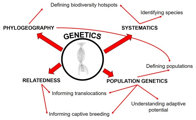
Since evolution is a constant process, occurring over both temporal and spatial scales, the impact of evolutionary history for current and future species cannot be overstated. The various forces of evolution through natural selection have strong, lasting impacts on the evolution of organisms, which is exemplified within the genetic make-up of all species. Phylogeography is the domain of research which intrinsically links this genetic information to historical selective environment (and changes) to understand historic distributions, evolutionary history, and even identify biodiversity hotspots.

The Ice Age(s)

Although there are a huge number of both historic and contemporary climatic factors that have influenced the evolution of species, one particularly important time period is referred to as the Pleistocene glacial cycles. The Pleistocene epoch spans from ~2 million years ago until ~100,000 years ago, and is a time of significant changes in the evolution of many species still around today (particularly for vertebrates). This is because the Pleistocene largely consisted of several successive glacial periods: at times, the climate was significantly cooler, glaciers were more widespread and sea-levels were lower (due to the deeper freezing of water around the poles). These periods were then followed by ‘interglacial periods’, where much of the globe warmed, ice caps melted and sea-levels rose. Sometimes, this natural pattern is argued as explaining 100% of recent climate change: don’t be fooled, however, as Pleistocene cycles were never as dramatic or irreversible as modern, anthropogenically-driven climate change.

Annotated glacial cycles.jpg — The general pattern of glacial and interglacial periods over the last 1 million years, adapted from Oceanbites.

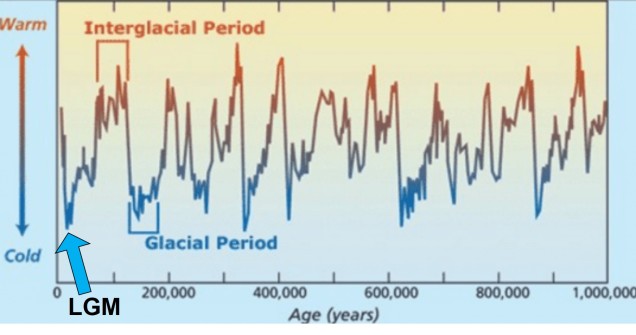
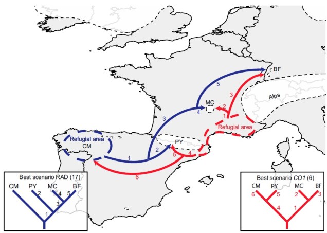
The glacial cycles of the Pleistocene had a number of impacts on a plethora of species on Earth. For many of these species, these glacial-interglacial periods resulted in what we call ‘glacial refugia’ and ‘interglacial expansion’: at the peak of glacial periods, many species’ distributions contracted to small patches of suitable habitat, like tiny islands in a freezing ocean. As the globe warmed during interglacial periods, these habitats started to spread and with them the inhabiting species. While it’s expected that this likely happened many times throughout the Pleistocene, the most clearly observed cycle would be the most recent one: referred to as the Last Glacial Maximum (LGM), at ~21,000 years ago. Thus, a quick dive into the literature shows that it is rife with phylogeographic examples of expansions and contractions related to the LGM.

glacial refugia example figure.jpg — An example of how phylogeographic analysis can find glacial refugia in species, in this case the montane caddisfly *Thremma gallicum* from Macher *et al.* (2017). The colours refer to the two datasets they used (blue = ddRADseq; red = mtDNA) and the arrows demonstrate migration pathways in the interglacial period following the LGM.

The glacial impact on genetic diversity

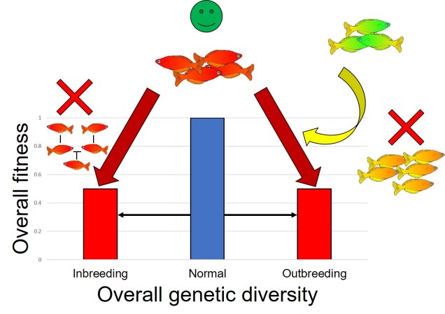
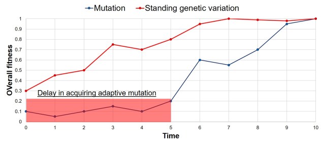
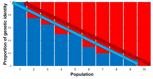
Why does any of this matter? Didn’t it all happen in the past? Well, that leads us back to the original point in this post: forces of evolution leave distinct impacts on the genetic architecture of species. In regards to glacial refugia, a clear pattern is often observed: populations occurring approximately in line with the refugia have maintained greater genetic diversity over time, whilst those in more unstable or unsuitable regions show much more reduced genetic diversity. And this makes sense: many of those populations likely went extinct during glaciation, and only within the last 20,000 or so years have been recolonised from nearby refugia. Accounting for genetic drift due to founder effect, it’s easy to see how this would cause genetic diversity to plummet.

Case study: the charismatic cheetah

And this loss of genetic diversity isn’t just a hypothetical, or an interesting note in evolution. It can have dire impacts for the survivability of species. Take for example, the very charismatic cheetah. Like many large, apex predator species, the cheetah in the modern day is endangered and at risk of extinction to a variety of threats, and although many of these are linked to modern activity (such as being killed to protect farms or habitat clearing), some of these go back much further in history.

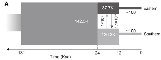
Believe it not, the cheetah as a species actually originated from an ancestor in the Americas: they’re closely related to other American big cats such as the puma/cougar. During the Miocene (5 – 8 million years ago), however, the ancestor of the modern cheetah migrated a very long way to Africa, diverging from its shared ancestor with jaguarandi and cougars. Subsequent migrations into Africa and Asia (where only the Iranian subspecies remains) during the Pleistocene, dated at ~100,000 and ~12,000 years ago, have been shown through whole genome analysis to have resulted in significant reductions in the genetic diversity of the cheetah. This timing correlates with the extinction of the cheetah and puma within North America, and the worldwide extinction of many large mammals including mammoths, dire wolves and sabre-tooth tigers.

cheetah bottleneck.jpg — The demographic history of the African cheetah population, based on whole genomes in Dobrynin *et al.* (2015). In this figure, ‘Eastern’ refers to a Tanzanian population whilst ‘southern’ refers to a Namibian population (and as such doesn’t depict bottlenecks elsewhere in the cheetah e.g. Iran). The initial population underwent a severe genetic bottleneck ~12,000 years ago, likely due to glaciation.

What does this mean for the cheetah? Well, the cheetah has one of the lowest amounts of genetic variation for any living mammal. It’s even lower than the Tasmanian Devil, a species with such notoriously low genetic diversity that a rampant face cancer (Devil Facial Tumour Disease) is transmissible simply because their immune system can’t recognise the transferred cancer cells as being different to the host animal. Similarly, for the cheetah, it’s possible to do reciprocal skin transplants without the likelihood of organ rejection simply because their immune system is incapable of determining the difference between foreign and host tissue cells.

cheetah diversity 2.jpg — Examples of the incredibly low genetic diversity in cheetah, both from Dobrynin *et al.* (2015). A) shows the relative level of genetic diversity in cheetah compared to many other species, being lower than Tasmanian Devils and significantly lower than humans and domestic cats. D) shows the overall variation across the genome of a domestic cat (top), the inbred Abyssinian cat (middle) and the cheetah (bottom). Highly variable regions are indicated in red, whilst low variability regions are indicated in green. As you can see, the entirety of the cheetah genome has incredibly low genetic variation, even compared to another cat species considered to have low genetic variation (the Abyssinian).

Inference for the future

Understanding the impact of the historic environment on the evolution and genetic diversity of living species is not just important for understanding how species became what they are today. It also helps us understand how species might change in the future, by providing the natural experimental evidence of evolution in a changing climate.

Rescuing the damselfish in distress: rescue or depression?

September 6, 2018September 6, 2018Sean Buckley7 Comments

Conservation management

Managing and conserving threatened and endangered species in the wild is a difficult process. There are a large number of possible threats, outcomes, and it’s often not clear which of these (or how many of these) are at play at any one given time. Thankfully, there are also a large number of possible conservation tools that we might be able to use to protect, bolster and restore species at risk.

Using genetics in conservation

Naturally, we’re going to take a look at the more genetics-orientated aspects of conservation management. We’ve discussed many times the various angles and approaches we can take using large-scale genetic data, some of which include:
• studying the evolutionary history and adaptive potential of species
• developing breeding programs using estimates of relatedness to increase genetic diversity
• identifying and describing new species for government legislation
• identifying biodiversity hotspots and focus areas for conservation
• identifying population boundaries for effective management/translocations

Genetics flowchart.jpg — An example of just some of the conservation applications of genetics research that we’ve talked about previously on *The G-CAT.*

This last point is a particularly interesting one, and an area of conservation research where genetics is used very often. Most definitions of a ‘population’ within a species rely on using genetic data and analysis (such as Fst) to provide a statistical value of how different groups of organisms are within said species. Ignoring some of the philosophical issues with the concept of a population versus a species due to the ‘speciation continuum’ (read more about that here), populations are often interpreted as a way to cluster the range of a species into separate units for conservation management. In fact, the most commonly referred to terms for population structure and levels are evolutionarily-significant units (ESUs), which are defined as a single genetically connected group of organisms that share an evolutionary history that is distinct from other populations; and management units (MUs), which may not have the same degree of separation but are still definably different with enough genetic data.

Hierarchy of structure.jpg — A diagram of the hierarchy of structure within a species. Remember that ESUs, by definition, should be evolutionary different from one another (i.e. adaptively divergent) whilst MUs are not necessarily divergent to the same degree.

This can lead to a particular paradigm of conservation management: keeping everything separate and pure is ‘best practice’. The logic is that, as these different groups have evolved slightly differently from one another (although there is often a lot of grey area about ‘differently enough’), mixing these groups together is a bad idea. Particularly, this is relevant when we consider translocations (“it’s never acceptable to move an organism from one ESU into another”) and captive breeding programs (“it’s never acceptable to breed two organisms together from different ESUs”). So, why not? Why does it matter if they’re a little different?

Outbreeding depression

Well, the classic reasoning is based on a concept called ‘outbreeding depression’. We’ve mentioned outbreeding depression before, and it is a key concept kept in mind when developing conservation programs. The simplest explanation for outbreeding depression is that evolution, through the strict process of natural selection, has pushed particularly populations to evolve certain genetic variants for a certain selective pressure. These can vary across populations, and it may mean that populations are locally adapted to a specific set of environmental conditions, with the specific set of genetic variants that best allow them to do this.

However, when you mix in the genetic variants that have evolved in a different population, by introducing a foreign individual and allowing them to breed, you essentially ‘tarnish’ the ‘pure’ gene pool of that population with what could be very bad (maladaptive) genes. The hybrid offspring of ‘native’ and this foreign individual will be less adaptive than their ‘pure native’ counterparts, and the overall adaptiveness of the population will decrease as those new variants spread (depending on the number introduced, and how negative those variants are).

Outbreeding depression example figure.jpg — An example of how outbreeding depression can affect a species. The original red fish population is not doing well- it is of conservation concern, and has very little genetic diversity (only the blue gene in this example). So, we decide to introduce new genetic diversity by adding in green fish, which have the orange gene. However, the mixture of the two genes and the maladaptive nature of the orange gene actually makes the situation worse, with the offspring showing less fitness than their preceding generations.

You might be familiar with inbreeding depression, which is based on the loss of genetic diversity from having too similar individuals breeding together to produce very genetically ‘weak’ offspring through inbreeding. Outbreeding depression could be thought of as the opposite extreme; breeding too different individuals introduced too many ‘bad’ alleles into the population, diluting the ‘good’ alleles.

Inbreeding vs outbreeding figure.jpg — An overly simplistic representation of how inbreeding and outbreeding depression can reduce overall fitness of a species. In inbreeding depression, the lack of genetic diversity due to related individuals breeding with one another makes them at risk of being unable to adapt to new pressures. Contrastingly, adding in new genes from external populations which aren’t fit for the target population can also reduce overall fitness by ‘diluting’ natural, adaptive allele frequencies in the population.

Genetic rescue

It might sound awfully purist to only preserve the local genetic diversity, and to assume that any new variants could be bad and tarnish the gene pool. And, surprisingly enough, this is an area of great debate within conservation genetics.

The counterpart to the outbreeding depression concerns is the idea of genetic rescue. For populations with already severely depleted gene pools, lacking the genetic variation to be able to adapt to new pressures (such as contemporary climate change), the situation seems incredibly dire. One way to introduce new variation, which might be the basis of new adaptation, bringing in individuals from another population of the same species can provide the necessary genetic diversity to help that population bounce back.

Genetic rescue example figure.jpg — An example of genetic rescue. This circumstance is identical to the one above, with the key difference being in the fitness of the introduced gene. The orange gene in this example is actually beneficial to the target population: by providing a new, adaptive allele for natural selection to act upon, overall fitness is increased for the red fish population.

The balance

So, what’s the balance between the two? Is introducing new genetic variation a bad idea, and going to lead to outbreeding depression; or a good idea, and lead to genetic rescue? Of course, many of the details surrounding the translocation of new genetic material is important: how different are the populations? How different are the environments (i.e. natural selection) between them? How well will the target population take up new individuals and genes?

Overall, however, the more recent and well-supported conclusion is that fears regarding outbreeding depression are often strongly exaggerated. Bad alleles that have been introduced into a population can be rapidly purged by natural selection, and the likelihood of a strongly maladaptive allele spreading throughout the population is unlikely. Secondly, given the lack of genetic diversity in the target population, most that need the genetic rescue are so badly maladaptive as it is (due to genetic drift and lack of available adaptive alleles) that introducing new variants is unlikely to make the situation much worse.

Purging and genetic rescue figure.jpg — An example of how introducing maladaptive alleles might not necessarily lead to decreased fitness. In this example, we again start with our low diversity red fish population, with only one allele (AA). To help boost genetic diversity, we introduce orange fish (with the TT allele) and green fish (with the GG allele) into the population. However, the TT allele is not very adaptive in this new environment, and individuals with the TT gene quickly die out (i.e. be ‘purged’). Individual with the GG gene, however, do well, and continue to integrate into the red population. Over time, these two variants will mix together as the two populations hybridise and overall fitness will increase for the population.

That said, outbreeding depression is not an entirely trivial concept and there are always limitations in genetic rescue procedures. For example, it would be considered a bad idea to mix two different species together and make hybrids, since the difference between two species, compared to two populations, can be a lot stronger and not necessarily a very ‘natural’ process (whereas populations can mix and disjoin relatively regularly).

The reality of conservation management

Conservation science is, at its core, a crisis discipline. It exists solely as an emergency response to the rapid extinction of species and loss of biodiversity across the globe. The time spent trying to evaluate the risk of outbreeding depression – instead of immediately developing genetic rescue programs – can cause species to tick over to the afterlife before we get a clear answer. Although careful consideration and analysis is a requirement of any good conservation program, preventing action due to almost paranoid fear is not a luxury endangered species can afford.

Origination of adaptation: the old and the new (genes)

September 1, 2018Sean Buckley3 Comments

Adaptation is arguably the most critical biological process in the evolution of species. The process of evolution by natural selection is the cornerstone of evolutionary biology (and indeed, all of contemporary biology!) and adaptation remains fundamental to the process. We know that adaptation is based on the idea that some genetic variants are ‘better’ adapted than others, and thus are unequally shared across a population. But where does this genetic variation come from?

The accumulation of new genetic variation

The classic way for new genetic variants to appear is often thought of as mutation: changes in a single base in the DNA are caused by various external processes such as chemical, physical or environmental influences (such as the sci-fi classics like UV rays or toxic chemicals). Although these forms of mutations happen very rarely and certainly don’t have the same effects comic books would leave you to believe, new mutations can occur relatively rapidly depending on the characteristics of the species. However, the most common way for new mutations to occur is actually part of the DNA replication process: copying DNA is not always perfect and even though the relevant proteins essentially run a spellcheck, sometimes the copy is not 100% perfect and new mutations occur.

Adaptation of mutation figure — An example of how adaptation can occur from a new mutation. In this example, we have one gene (TTXTT), with initial only one allele (variant), TTATT. In the second generation (row), a mutation occurs in one individual which creates a new, second allele: TTGTT. This allele is favoured over the TTATT allele, and in the next generation it’s frequency increases as the alternative allele frequency decreases (the pattern is shown in the frequency values on the right side).

It is important to remember that only mutations that are present in the reproductive cells (sperm and eggs) can be inherited and passed on, and thus be a source for adaptation. Mutations in other tissues of the body, such as within the skin, are not spread across the entire body of the subject and thus aren’t passed on to offspring.

Standing genetic variation

Alternatively, genetic variation might already be present within a species or population. This is more likely if population sizes are large and populations are well connected and interbreeding. We refer to this diverse initial gene pool as ‘standing genetic variation’: that is, the amount of genetic variation within the population or species before the selective pressure requiring adaptation. Standing genetic variation can be thought of as the ‘diversity of choices’ for natural selection to act upon: the variants are readily available, and if a good choice exists it will be favoured by natural selection and become more widespread within the population or species (i.e. evolve).

Adaptation of standing variation figure.jpg — A slightly more complex example of how adaptation can occur from standing variation, this time with two different genes. One codes for fur colour, with two different alleles: GCATA codes for orange fur, and GCGTA codes for grey fur. The other gene codes for ear tufts, with TTCCT coding for tufts and TCCCT coding for no tufts. Natural selection favours both orange fur and tufted ears, and cats with these traits reproduce more frequently than those without (see graph below). These cats probably look familiar.

Graph of standing variation.jpg — The frequency of all four alleles (i.e. either allele for both genes) over the generations in the above figure. Clearly, we can see how adaptation rapidly favours orange fur and tufted ears over grey fur and non-tufted ears with the shifts in frequencies over the different alleles.

We’ve discussed standing genetic variation before on The G-CAT, but often in a different light (and phrasing). For example, when we’ve talked about founder effect: that is, when a population is formed from only a few different individuals which causes it to be very genetically depauperate. In populations under strong founder effect, there is very little standing genetic variation for natural selection to act upon. This has long been an enigma for many pest species: how have they managed to proliferate so widely when they often originate from so few individuals and lack genetic diversity?

Adaptive variation

Adaptation may not require new genetic variants to be generated from mutation. If there are a large number of alleles within the gene pool to start with, then natural selection may favour one of those variants over others and allow adaptation to start immediately. Compared to the rate at which new mutations occur, are potentially corrected for in DNA repair, are potentially erased by genetic drift, and then put under selective pressure, adaptation from standing genetic variation can occur very quickly.

Rate of adaptation figure.jpg — A rough example of the speed of adaptation depending on how the adaptive allele originated: whether it was already present (in the form of standing variation), or whether it was created by a new mutation. As one would expect, there is a significant lag delay in adaptation in the mutation scenario, based on the time it takes for said adaptive mutation to be created through relatively random processes. Thus, a positively selected allele from standing variation can allow a species to adapt much faster than waiting for a positive mutation to occur.

Conserving genetic variation

Given the adaptive potential provided by maintaining a good amount of standing genetic variation, it is imperative to conserve genetic diversity within populations in conservation efforts. This is why we often equate genetic diversity with ‘adaptive potential’ of species, although the exact amount of genetic diversity required for adaptive potential depends on a large number of other factors. Clearly, in some instances species show the ability to adapt to new pressures or novel environments even without a large amount of standing genetic variation.

It is important to remember that standing genetic variation consists of two types: neutral genetic diversity, which is not necessarily under selection at the time, and adaptive genetic diversity, which is directly under selection (although this can be either for or against the given variant). However, currently neutral genetic variants may become adaptive variants in the future if selective pressures change: although those different variants aren’t necessarily beneficial or detrimental at the moment, that may change in the future. Thus, conserving both types of genetic diversity is important for the survivability and longevity of populations under conservation programs.

Other types of adaptation

Although genetic diversity is clearly critically important for adaptive potential, alternative mechanisms for adaptation also exist. One of these relies less on the actual genetic variants being different, but rather how individual genes are used. This can happen in a few different ways, but mostly commonly this is through alternative splicing: when a gene is being ‘read’ and a protein is produced, different parts of the gene can be used (and in different order) to make a completely different protein.

Alternate splicing figure.jpg — An extreme example of alternate splicing of one gene. We start with a single gene, composed of 5 (A–E) main gene elements (exons). Different environmental pressures (like fire risk, flooding, cold weather or predators, for example) cause the organism to use different combinations of these exons to make different proteins (right side; A–D). Actual alternate splicing is not usually this straight-forward (one gene doesn’t conveniently split into four forms depending on the threat), but the process is generally the same.

Believe it or not, we’ve sort of discussed the effects of alternative splicing before. Phenotypic plasticity occurs when a single organism can have very different physiological traits depending on the environment: even though the genes are the same, they are utilised in different ways to make a different body shape. This is how some species can look incredibly different when they live in different places even if they’re genetically very similar. That said, for the vast majority of species maintaining good levels of genetic diversity is critical for the survivability of said species.

It takes (at least) two: coevoultion and species interactions

August 24, 2018August 24, 2018Sean Buckley1 Comment

The environmental context of adaptation

We’ve talked many times before about how species evolve in response to some kind of environmental pressure, which favours (or disfavours) certain traits within that species. Over time, this drives changes in the frequencies of species traits and alters the overall average phenotype of that species (sometimes slowly, sometimes rapidly).

While we usually talk about the environment in terms of abiotic conditions such as temperature or climate, biotic factors are equally important: that is, the parts of the environment which are themselves also alive. Because of this, changes in one species can have profound repercussions on other species linked within the ecosystem. Thus, the evolution of one species is intrinsically linked to the evolution of other relevant species within the ecosystem: often, these connected evolutionary pathways battle with one another as each one changes. Let’s take a look at a few different examples of how evolution of one species may impact the evolution of another.

Predator-prey coevolution

One of the most obvious ways the evolution of two different species can interact is in predator and prey relationships. Naturally, prey species evolve to be able to defend themselves from predators in various ways, such as crypsis (e.g. camouflage), toxicity or behavioural changes (such as nocturnalism or group herding). Contrastingly, predators will evolve new and improved methods for detecting and hunting prey, such as enhanced senses, venom and stealth (through soft-padded feet, for example).

There are millions of possible examples of predator-prey coevolution that could be used as examples here, based on the continual drive for one species to get the upper hand over the other. But one that comes to mind is of a creature that I learnt about while on holiday in Scandinavia: the pine marten, and how it affects squirrels.

This photo is one that I took whilst on a lunch break at a bakery in the Norwegian mountains, of a small critter running among the rocks by the lakeside. Not sure exactly what species it was, I asked the tour director who excitedly told me that it was a pine marten. After doing a bit of research on them (and trying to figure out what the difference between a pine marten, a stoat, and a weasel is), I’ve discovered that it’s actually more likely to be a stoat than a pine marten, based on size and colour. But pine martens are still an intriguing species in their own right (and also found in Norway, so the confusion is understandable).

The pine marten is a species in the mustelid family, along with otters, weasels, stoats, and wolverines. Like many mustelids, they are carnivorous mammals which feed on a variety of different prey items like rodents, small birds and insects. One of the more abundant species that they prey upon are squirrels: both red squirrels and grey squirrels are potential food for the cute yet savage pine marten.

However, within the distribution of pine martens (across much of Europe), red squirrels are the native species and grey squirrels are invasive, originating from North America. Because of the long-lasting relationship between red squirrels and pine martens, they’ve co-evolved: most notably, by red squirrels changing to a mostly arboreal lifestyle and avoiding the ground as much as possible. Grey squirrels, however, have not had the evolutionary history to learn this lesson and are easy food for a smart pine marten. Thus, in regions where pine martens have been conserved or reintroduced, they are actively controlling the invasive grey squirrel population, which in turn boosts the native red squirrel population by reduction of competition. The coevolutionary link between red squirrels and pine martens is critical for combating the invasive species.

Martens and squirrels figure.jpg — The relationship between pine marten abundance and the abundance of both red (native) and grey (invasive) squirrels. On the left, without pine martens the invasive species runs rampant, outcompeting the native species. However, as pine martens increase in the ecosystem, the grey squirrels are predated on much more than the red squirrels due to their naivety, leading to the ‘natural’ balance on the right.

Martens and squirrels stats.jpg — A diagram of how the abundance of squirrels changes relative to the number of pine martens. The invasive grey squirrels are significantly depleted by pine marten presence, which in turn allows the native red squirrels to increase in population size after being freed from competition.

Host-parasite coevolution

In a similar vein to predator and prey coevolution, pathogenic species and their unfortunate hosts also undergo a sort of ‘arms race’. Parasites must keep evolving new ways to infect and transmit to hosts as the hosts evolve new methods of resisting and avoiding the infecting species. This spiralling battle of evolutionary forces is dubbed as the ‘Red Queen hypothesis’, formulated in 1973 by Leigh Van Valen and used to describe many other forms of coevolution. The name comes from Lewis Carroll’s Through the Looking Glass, and one quote in particular:

‘Now, here, you see, it takes all the running you can do, to keep in the same place’.

The quote references how species must continually adapt and respond to the evolution of other species just keep existing and prevent extinction. Species that remain static and stop evolving will inevitably go extinct as the world around them changes.

Mimicry

Plenty of other strange and unique mechanisms of coevolution exist within nature. One of them is mimicry, the process by which one species attempts to look like another to protect itself. The most iconic group known for this is butterflies: many species, although they may be evolutionarily very different, share similar colouration patterns and body shapes as mimics. Depending on the nature of the copy, mimicry can be classified into two broad categories. In either case, the initial ‘reference’ species is toxic or unpalatable to predators and uses a type of colour signal to communicate this: think of the bright yellow colours of bees and wasps or the red of ladybirds. Where the two categories change is in the nature of the ‘mimic’ species.

Müllerian mimicry

If the mimic is also toxic or unpalatable, we call this Müllerian mimicry (after Johann Friedrich Theodor Müller). By sharing the same colouration patterns and both being toxic, the two mimicking species boost the potential for the signal to be learnt by predators. If a predator eats either species, it will associate that colour pattern with toxicity and neither species are as likely to be preyed upon in the future. In this sense, it is a cooperative coevolutionary relationship between the two physically similar species.

Mullerian mimicry figure — A (somewhat familiar) example of Müllerian mimicry with two species of butterflies, the monarch and the viceroy. Although this has traditionally been thought of as a textbook case of Batesian mimicry (see below), the toxicity of both species likely makes it a scenario of Müllerian mimicry instead. Since both butterflies share the same pattern and both are toxic, it sends a strong signal to predators such as wasps to avoid them both.

Batesian mimicry

In contrast, the mimic might not actually be toxic or unpalatable, and simply copying a toxic species. This is referred to as Batesian mimicry (after Henry Walter Bates), and involves a mimic species relying on the association of colour and toxicity to have been learnt by predators through the ‘reference’ species. Although the mimic is not toxic, it is essentially piggy-backing on the hard evolutionary work that has already been done by the actually toxic species. In this case, the coevolutionary relationship is more parasitic as the mimic benefits from the ‘reference’ but the favour is not returned.

Coevolution of species and the importance of species interactions

There are countless of other species interactions which could drive coevolutionary relationships in nature. These can include various forms of symbiosis, or the response of different species to ecosystem engineers: that is, species that can change and shape the environment around them (such as corals in reef systems). Understanding how a species evolves within its environment thus needs to consider how many other local species are also evolving and responding in their own ways.

Moving right along: dispersal and population structure

July 25, 2018July 24, 2018Sean Buckley9 Comments

The impact of species traits on evolution

Although we often focus on the genetic traits of species in molecular ecology studies, the physiological (or phenotypic) traits are equally as important in shaping their evolution. These different traits are not only the result themselves of evolutionary forces but may further drive and shape evolution into the future by changing how an organism interacts with the environment.

There are a massive number of potential traits we could focus on, each of which could have a large number of different (and interacting) impacts on evolution. One that is often considered, and highly relevant for genetic studies, is the influence of dispersal capability.

Dispersal

Dispersal is essentially the process of an organism migrating to a new habitat, to the point of the two being used almost interchangeably. Often, however, we regard dispersal as a migration event that actually has genetic consequences; particularly, if new populations are formed or if organisms move from one population to another. This can differ from straight migration in that animals that migrate might not necessarily breed (and thus pass on genes) into a new region during their migration; thus, evidence of those organisms will not genetically proliferate into the future through offspring.

Naturally, the ability of organisms to disperse is highly variable across the tree of life and reliant on a number of other physiological factors. Marine mammals, for example, can disperse extremely far throughout their lifetimes, whereas some very localised species like some insects may not move very far within their lifetime at all. The movement of organisms directly facilitates the movement of genetic material, and thus has significant impacts on the evolution and genetic diversity of species and populations.

Dispersal vs pop structure — The (simplistic) relationship between dispersal capability and one aspect of population genetics, population structure (measured as Fst). As organisms are more capable of dispersing longer distance (or more frequently), the barriers between populations become weaker.

Highly dispersive species

At one end of the dispersal spectrum, we have highly dispersive species. These can move extremely long distances and thus mix genetic material from a wide range of habitats and places into one mostly-cohesive population. Because of this, highly dispersive species often have strong colonising abilities and can migrate into a range of different habitats by tolerating a wide range of conditions. For example, a single whale might hang around Antarctica for part of the year but move to the tropics during other times. Thus, this single whale must be able to tolerate both ends of the temperature spectrum.

As these individuals occupy large ranges, localised impacts are unlikely to critically affect their full distribution. Individual organisms that are occupying an unpleasant space can easily move to a more favourable habitat (provided that one exists). Furthermore, with a large population (which is more likely with highly dispersive species), genetic drift is substantially weaker and natural selection (generally) has a higher amount of genetic diversity to work with. This is, of course, assuming that dispersal leads to a large overall population, which might not be the case for species that are critically endangered (such as the cheetah).

Highly dispersive animals often fit the “island model” of Wright, where individual subpopulations all have equal proportions of migrants from all other subpopulations. In reality, this is rare (or unreasonable) due to environmental or physiological limitations of species; distance, for example, is not implicitly factored into the basic island model.

Intermediately dispersing species

A large number of species, however, are likely to occupy a more intermediate range of dispersal ability. These species might be able to migrate to neighbouring populations, or across a large proportion of their geographic range, but individuals from one end of the range are still somewhat isolated from individuals at the other end.

This often leads to some effect of population structure; different portions of the geographic range are genetically segregated from one another depending on how much gene flow (i.e. dispersal) occurs between populations. In the most simplest scenario, this can lead to what we call isolation-by-distance. Rather than forming totally independent populations, gene flow occurs across short ranges between adjacent ‘populations’. This causes a gradient of genetic differentiation, with one end of the range being clearly genetically different to the other end, with a gradual slope throughout the range. We see this often in marine invertebrates, for example, which might have somewhat localised dispersal but still occupy a large range by following oceanographic currents.

River IDB network — An example of how an isolation-by-distance population network might come about. In this example, we have a series of populations (the different pie charts) spread throughout a river system (that blue thing). The different pie charts represent how much of the genetics of that population matches one end of the river: either the blue end (left) or red end (right). Populations can easily disperse into adjacent populations (the green arrows) but less so to further populations. This leads to gradual changes across the length of the river, with the far ends of the river clearly genetically distinct from the opposite end but relatively similar to neighbouring populations.

River IDB pop structure.jpg — The genetic representation of the above isolation-by-distance example. Each column represents a single population (in the previous figure, a pie chart), with the different colours also representing the relative genetic identity of that population. As you can see, moving from Population 1 to 10 leads to a gradient (decreasing) in blue genes but increase in red genes. The inverse can be said moving in the opposite direction. That said, comparing Population 1 and Population 10 shows that they’re clearly different, although there is no clear cut-off point across the range of other populations.

Medium dispersal capabilities are also often a requirement for forming ‘metapopulations’. In this population arrangement, several semi-independent populations are present within the geographic range of the species. Each of these are subject to their own local environmental pressures and demographic dynamics, and because of this may go locally extinct at any given time. However, dispersal connections between many of these populations leads to recolonization and gene flow patterns, allowing for extinction-dispersal dynamics to sustain the overall metapopulation. Generally, this would require greater levels of dispersal than those typically found within metapopulation species, as individuals must traverse uninhabitable regions relatively frequently to recolonise locally extinct habitat.

Metapopulation structure.jpg — An example of metapopulation dynamics. Different subpopulations (lettered circles) are connected via dispersal (arrows). These different subpopulations can be different sizes and are mostly independent of one another, meaning that a single subpopulation can go locally extinct (the red X) without collapsing the entire system. The different dispersal pathways mean that one population can recolonise extinct habitat and essentially ‘rebirth’ other subpopulations (the green arrows).

Weakly dispersing species

At the far opposite end of the dispersal ability spectrum, we have low dispersal species. These are often localised, endemic species that for various reasons might be unable to travel very far at all; for some, they may spend their entire adult life in a sedentary form. The lack of dispersal lends to very strong levels of population structure, and individual populations often accumulate genetic differences relatively quickly due to genetic drift or local adaptation.

Species with low dispersal capabilities are often at risk of local extinction and are unable to easily recolonise these habitats after the event has ended. Their movement is often restricted to rare environmental events such as flooding that carry individuals long distances despite their physiological limitations. Because of this, low dispersal species are often at greater risk of total extinction and extinction vertices than their higher dispersing counterparts.

Accounting for dispersal in population genetics

Incorporating biological and physiological aspects of our study taxa is important for interpreting the evolutionary context of species. Dispersal ability is but one of many characteristics that can influence the ability of species to respond to selective pressures, and the context in which this natural selection occurs. Thus, understanding all aspects of an organism is important in building the full picture of their evolution and future prospects.