A fellow science student once drunkenly said that “I am a biologist…I don’t understand art.” Although somewhat bemusing (both in and out of context), it raises a particular philosophical idea that I can’t agree with: that art and science directly contradict one another.
It’s a somewhat clichéd paradigm that art and science must work at odds with one another. The idea that art embraces emotion, creativity and abstract perception whilst science is solely dictated by rationality, methodology and universal statistics is one that still seems to be somewhat pervasive throughout society and culture. While there seems to be a more recent shift against this, with both ends of the spectrum acknowledging the importance of the other in their respective fields, the intersection of art and science has a long and productive history.
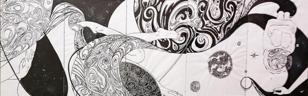
A piece I did for a high school assignment some years ago. The artwork was meant to be the visual representation of Edgar Allen Poe’s 1829 poem “Sonnet- To Science“, by showing the dichotomy of the beauty of the natural world (left) vs. the cold, rigorousness of science (right).
Typically, the disjunction from the emotional and evocative state of people with science is through how the science is written. In many formats (particularly for the most widely used scientific journals), artistic and emotional writing is seen to detract from the overall message and objectivity of the piece itself. And while appeal to emotion can certainly take away from or mislead the message of the writing, it’s important to connect and attract readers to the work in the first place. Trying to find a possible avenue to work in personal style and artistry into an academic paper is an incredibly difficult affair. This is a large contributor to the merit of non-journalistic forms of scientific communication such as books, poetry and even blogs (this was one motivator in starting this blog, in fact).
It might come as a surprise to readers that I love art quite a lot, especially given the (lack of) quality of the drawings in this blog. But I’ve always tried to flex my creative side and particular when I was a younger was a more avid writer and sketcher. And that truth of the matter is that I don’t feel that the artistic side of a person has to be at odds with their scientific side. In fact, the two directly complement each other by linking our rational, objective understanding of the world with the emotional, expressive and ideological aspects of the human personality.
My own (non-blog) artwork tends to combine both imagery from the natural world and more emotional themes (e.g. mental health).
The art of science
From one angle, science is actively driven by creativity, ambition and often abstract ideation. The desire to delve deep to find new knowledge is intrinsically an emotional and philosophical process and to pretend that science is devoid of passion discredits both the research and the researcher. Entire disciplines of biology, for example, find themselves driven by science and people with deep emotional connections to the natural world and a desire to both understand and protect the diversity of life. The works of John Gould in his explorations of the Australian biota remain some of my favourites for both scientific and artistic merit.
The science of art
From the other direction, science can also inform artistic works by expanding the human knowledge and experience with which to draw inspiration from. Naturally, this is an intrinsic part of genres such as science fiction, but many works of horror, abstraction, fantasy, thriller also draw on theories and revolutions brought about by scientific discovery. The further we understand the processes of the universe through scientific discovery, the greater the context and extent of our philosophical and emotional perspectives can be allowed to vary.
A piece by local artist and good friend of mine (and also the designer of The G-CAT logo!) Michelle Fedornak. She describes her piece (dubbed ‘We Are All Stars’) as inspired by the explorations of the Mars Curiosity rover and tackles themes of identity and isolation in the galactic space. Thus, her work combines the philosophical and emotional side of scientific exploration with the artistry and consciousness of human identity.
Unity
Gone are the days of dichotomy between 18-19th Century Impressionism and Enlightenment. Instead, the unity of science and art in the modern world can have significant positive contributions to both fields. Although there are still some elements of resistance between the two avenues, it is my belief that by allowing the intrinsically emotional nature of science to be expressed (albeit moderated by reason and logic) will allow science to influence a greater number of people, an especially important connection in the age of cynicism.
Understanding the evolutionary history of species can be a complicated matter, both from theoretical and analytical perspectives. Although phylogenetics addresses many questions about evolutionary history, there are a number of limitations we need to consider in our interpretations.
One of these limitations we often want to explore in better detail is the estimation of the divergence times within the phylogeny; we want to know exactly when two evolutionary lineages (be they genera, species or populations) separated from one another. This is particularly important if we want to relate these divergences to Earth history and environmental factors to better understand the driving forces behind evolution and speciation. A traditional phylogenetic tree, however, won’t show this: the tree is scaled in terms of the genetic differences between the different samples in the tree. The rate of genetic differentiation is not always a linear relationship with time and definitely doesn’t appear to be universal.
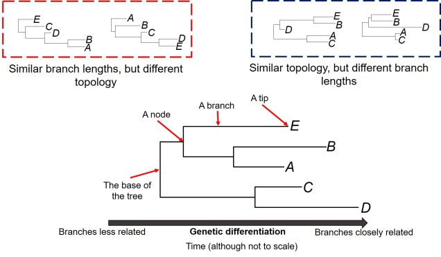
The general anatomy of a phylogenetic tree. A phylogeny describes the relationships of tips (i.e. which are more closely related than others; referred to as the topology), how different these tips are (the length of the branches) and the order they separated in time (separations shown by the nodes). Different trees can share some traits but not others: the red box shows two phylogenetic trees with similar branch lengths (all of the branches are roughly the same) but different topology (the tips connect differently: A and B are together on the left but not on the right, for example). Conversely, two trees can have the same topology, but show differing lengths in the branches of the same tree (blue box). Note that the tips are all in the same positions in these two trees. Typically, it’s easier to read a tree from right to left: the two tips who have branches that meet first are most similar genetically; the longer it takes for two tips to meet along the branches, the less similar they are genetically.
How do we do it?
The parameters
There are a number of parameters that are required for estimating divergence times from a phylogenetic tree. These can be summarised into two distinct categories: the tree model and the substitution model.
The first one of these is relatively easy to explain; it describes the exact relationship of the different samples in our dataset (i.e. the phylogenetic tree). Naturally, this includes the topology of the tree (which determines which divergences times can be estimated for in the first place). However, there is another very important factor in the process: the lengths of the branches within the phylogenetic tree. Branch lengths are related to the amount of genetic differentiation between the different tips of the tree. The longer the branch, the more genetic differentiation that must have accumulated (and usually also meaning that longer time has occurred from one end of the branch to the other). Even two phylogenetic trees with identical topology can give very different results if they vary in their branch lengths (see the above Figure).
The second category determines how likely mutations are between one particular type of nucleotide and another. While the details of this can get very convoluted, it essentially determines how quickly we expect certain mutations to accumulate over time, which will inevitably alter our predictions of how much time has passed along any given branch of the tree.
Calibrating the tree
However, at least one another important component is necessary to turn divergence time estimates into absolute, objective times. An external factor with an attached date is needed to calibrate the relative branch divergences; this can be in the form of the determined mutation rate for all of the branches of the tree or by dating at least one node in the tree using additional information. These help to anchor either the mutation rate along the branches or the absolute date of at least one node in the tree (with the rest estimated relative to this point). The second method often involves placing a time constraint on a particular node of the tree based on prior information about the biogeography of the species (for example, we might know one species likely diverged from another after a mountain range formed: the age of the mountain range would be our constraints). Alternatively, we might include a fossil in the phylogeny which has been radiocarbon dated and place an absolute age on that instead.
Don’t you know it’s rude to ask an ammomite her age?
In regards to the former method, mutation rates describe how fast genetic differentiation accumulates as evolution occurs along the branch. Although mutations gradually accumulate over time, the rate at which they occur can depend on a variety of factors (even including the environment of the organism). Even within the genome of a single organism, there can be variation in the mutation rate: genes, for example, often gain mutations slower than non-coding region.
Although mutation rates (generally in the form of a ‘molecular clock’) have been traditionally used in smaller datasets (e.g. for mitochondrial DNA), there are inherent issues with its assumptions. One is that this rate will apply to all branches in a tree equally, when different branches may have different rates between them. Second, different parts of the genome (even within the same individual) will have different evolutionary rates (like genes vs. non-coding regions). Thus, we tend to prefer using calibrations from fossil data or based on biogeographic patterns (such as the time a barrier likely split two branches based on geological or climatic data).
The analytical framework
All of these components are combined into various analytical frameworks or programs, each of which handle the data in different ways. Many of these are Bayesian model-based analysis, which in short generates hypothetical models of evolutionary history and divergence times for the phylogeny and tests how well it fits the data provided (i.e. the phylogenetic tree). The algorithm then alters some aspect(s) of the model and tests whether this fits the data better than the previous model and repeats this for potentially millions of simulations to get the best model. Although models are typically a simplification of reality, they are a much more tractable approach to estimating divergence times (as well as a number of other types of evolutionary genetics analyses which incorporating modelling).
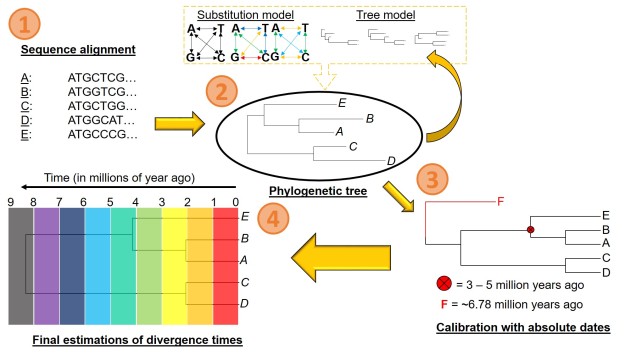
A (believe it or not, simplified) pipeline for estimating divergence times from a phylogeny. 1) We obtain our DNA sequences for our samples: in this example, we’ll see each Sample (A-E) is a representative of a single species. We align these together to make sure we’re comparing the same part of the genome across all of them. 2) We estimate the phylogenetic tree for our samples/species. In a Bayesian framework, this means creating simulation models containing a certain substitution model and a given tree model (containing certain topology and branch lengths). Together, these two models form the likelihood model: we then test how well this model explains our data (i.e. the likelihood of getting the patterns in our data if this model was true). We repeat these simulations potentially hundreds of thousands of times until we pinpoint the most likely model we can get. 3) Using our resulting phylogeny, we then calibrate some parts of it based on external information. This could either be by including a carbon-dated fossil (F) within the phylogeny, or constraining the age of one node based on biogeographic information (the red circle and cross). 4) Using these calibrations as a reference, we then estimated the most likely ages of all the splits in the tree, getting our final dated phylogeny.
Despite the developments in the analytical basis of estimating divergence times in the last few decades, there are still a number of limitations inherent in the process. Many of these relate to the assumptions of the underlying model (such as the correct and accurate phylogenetic tree and the correct estimations of evolutionary rate) used to build the analysis and generate simulations. In the case of calibrations, it is also critical that they are correctly dated based on independent methods: inaccurate radiocarbon dating of a fossil, for example, could throw out all of the estimations in the entire tree. That said, these factors are intrinsic to any phylogenetic analysis and regularly considered by evolutionary biologists in the interpretations and discussions of results (such as by including confidence intervals of estimations to demonstrate accuracy).
Understanding the temporal aspects of evolution and being able to relate them to a real estimate of age is a difficult affair, but an important component of many evolutionary studies. Obtaining good estimates of the timing of divergence of populations and species through molecular dating is but one aspect in building the picture of the history of all organisms, including (and especially) humans.
While evolutionary genetics studies often focus on the underlying genetic architecture of species and populations to understand their evolution, we know that natural selection acts directly on physical characteristics. We call these the phenotype; by studying changes in the genes that determine these traits (the genotype), we can take a nuanced approach at studying adaptation. However, our ability to look at genetic changes and relate these to a clear phenotypic trait, and how and why that trait is under natural selection, can be a difficult task.
One gene for one trait
The simplest (and most widely used) models of understanding the genetic basis of adaptation assume that a single genotype codes for a single phenotypic trait. This means that changes in a single gene (such as outliers that we have identified in our analyses) create changes in a particular physical trait that is under a selective pressure in the environment. This is a useful model because it is statistically tractable to be able to identify few specific genes of very large effect within our genomic datasets and directly relate these to a trait: adding more complexity exponentially increases the difficulty in detecting patterns (at both the genotypic and phenotypic level).
An example of a single gene coding for a single phenotypic trait. In this example, the different combination of alleles of the one gene determines the colour of the cat.
Many genes for one trait: polygenic adaptation
Unfortunately, nature is not always convenient and recent findings suggest that the overwhelming majority of the genetics of adaptation operate under what is called ‘polygenic adaptation’. As the name suggestions, under this scenario changes (even very small ones) in many different genes combine together to have a large effect on a particular phenotypic trait. Given the often very small magnitude of the genetic changes, it can be extremely difficult to separate adaptive changes in genes from neutral changes due to genetic drift. Likewise, trying to understand how these different genes all combine into a single functional trait is almost impossible, especially for non-model species.
Polygenic adaptation is often seen for traits which are clearly heritable, but don’t show a single underlying gene responsible. Previously, we’ve covered this with the heritability of height: this is one of many examples of ‘quantitative trait loci’ (QTLs). Changes in one QTL (a single gene) causes a small quantitative change in a particular trait; the combined effect of different QTLs together can ‘add up’ (or counteract one another) to result in the final phenotype value.
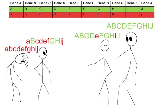
An example of polygenic quantitative trait loci. In this example, height is partially coded for by a total of ten different genes: the dominant form of each gene (Capitals, green) provides more height whereas the recessive form (lowercase, red) doesn’t. The cumulative total of these components determines how tall the person is: the person on the far right was very unlucky and got 0/10 height bonuses and so is the shortest. Progressively from left to right, some genes are contributing to the taller height of the people, with the far right person standing tall with the ultimate 10/10 pro-height genes. For reference, height is actually likely to be coded for by thousands of genes, not 10.
The mechanisms which underlie polygenic adaptation can be more complex than simple addition, too. Individual genes might cause phenotypic changes which interact with other phenotypes (and their underlying genotypes) to create a network of changes. We call these interactions ‘epistasis’, where changes in one gene can cause a flow-on effect of changes in other genes based on how their resultant phenotypes interact. We can see this in metabolic pathways: given that a series of proteins are often used in succession within pathways, a change in any single protein in the process could affect every other protein in the pathway. Of course, knowing the exact proteins coded for every gene, including their physical structure, and how each of those proteins could interact with other proteins is an immense task. Similar to QTLs, this is usually limited to model species which have a large history of research on these specific areas to back up the study. However, some molecular ecology studies are starting to dive into this area by identifying pathways that are under selection instead of individual genes, to give a broader picture of the overall traits that are underlying adaptation.
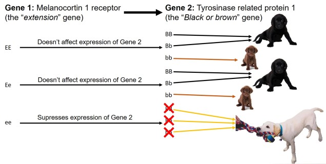
My favourite example of epistasis on coat colour in labradors. Two genes together determine the colour of the coat, with strong interactions between them. The first gene (E/e) determines whether or not the underlying coat gene (B/b) is masked or not: two recessive alleles of the first gene (ee) completely blocks Gene 2 and causes the coat to become golden regardless of the second gene genotype (much like my beloved late childhood pet pictured, Sunny). If the first gene has at least one dominant allele, then the second gene is allowed to express itself. Possessing a dominant allele (BB or Bb) leads to a black lab; possessing two recessive alleles (bb) makes a choc lab!The possible combinations of genotypes for the two above genes and the resultant coat colour (indicated by the box colour).
One gene for many traits: pleiotropy and differential gene expression
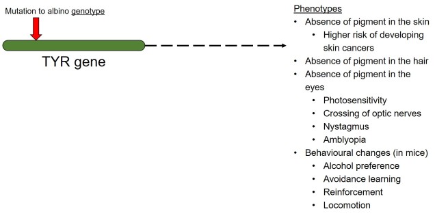
In contrast to polygenic traits, changes in a single gene can also potentially alter multiple phenotypic traits simultaneously. This is referred to as ‘pleiotropy’ and can happen if a gene has multiple different functions within an organism; one particular protein might be a component of several different systems depending on where it is found or how it is arranged. A clear example of pleiotropy is in albino animals: the most common form of albinism is the result of possessing two recessive alleles of a single gene (TYR). The result of this is the absence of the enzyme tyrosinase in the organism, a critical component in the production of melanin. The flow-on phenotypic effects from the recessive gene most obviously cause a lack of pigmentation of the skin (whitening) and eyes (which appear pink), but also other physiological changes such as light sensitivity or total blindness (due to changes in the iris). Albinism has even been attributed to behavioural changes in wild field mice.
A very simplified diagram of how one genotype (the albino version of the TYR gene) can lead to a large number of phenotypic changes via pleiotropy (although many are naturally physiologically connected).
Because pleiotropic genes code for several different phenotypic traits, natural selection can be a little more complicated. If some resultant traits are selected against, but others are selected for, it can be difficult for evolution to ‘resolve’ the balance between the two. The overall fitness of the gene is thus dependent on the balance of positive and negative fitness of the different traits, which will determine whether the gene is positively or negatively selected (much like a cost-benefit scenario). Alternatively, some traits which are selectively neutral (i.e. don’t directly provide fitness benefits) may be indirectly selected for if another phenotype of the same underlying gene is selected for.
Multiple phenotypes from a single ‘gene’ can also arise by alternate splicing: when a gene is transcribed from the DNA sequence into the protein, the non-coding intron sections within the gene are removed. However, exactly which introns are removed and how the different coding exons are arranged in the final protein sequence can give rise to multiple different protein structures, each with potentially different functions. Thus, a single overarching gene can lead to many different functional proteins. The role of alternate splicing in adaptation and evolution is a rarely explored area of research and its importance is relatively unknown.
Non-genes for traits: epigenetics
This gets more complicated if we consider ‘non-genetic’ aspects underlying the phenotype in what we call ‘epigenetics’. The phrase literally translates as ‘on top of genes’ and refers to chemical attachments to the DNA which control the expression of genes by allowing or resisting the transcription process. Epigenetics is a relatively new area of research, although studies have started to delve into the role of epigenetic changes in facilitating adaptation and evolution. Although epigenetics is still a relatively new research topic, future research into the relationship between epigenetic changes and adaptive potential might provide more detailed insight into how adaptation occurs in the wild (and might provide a mechanism for adaptation for species with low genetic diversity)!
The different interactions between genotypes, phenotypes and fitness, as well as their complex potential outcomes, inevitably complicates any study of evolution. However, these are important aspects of the adaptation process and to discard them as irrelevant will not doubt reduce our ability to examine and determine evolutionary processes in the wild.
One of the most fundamental aspects of natural selection and evolution is, of course, the underlying genetic traits that shape the physical, selected traits. Most commonly, this involves trying to understand how changes in the distribution and frequencies of particular genetic variants (alleles) occur in nature and what forces of natural election are shaping them. Remember that natural selection acts directly on the physical characteristics of species; if these characteristics are genetically-determined (which many are), then we can observe the flow-on effects on the genetic diversity of the target species.
Although we might expect that natural selection is a fairly predictable force, there are a myriad of ways it can shape, reduce or maintain genetic diversity and identity of populations and species. In the following examples, we’re going to assume that the mentioned traits are coded for by a single gene with two different alleles for simplicity. Thus, one allele = one version of the trait (and can be used interchangeably). With that in mind, let’s take a look at the three main broad types of changes we observe in nature.
Directional selection
Arguably the most traditional perspective of natural selection is referred to as ‘directional selection’. In this example, nature selection causes one allele to be favoured more than another, which causes it to increase dramatically in frequency compared to the alternative allele. The reverse effect (natural selection pushing against a maladaptive allele) is still covered by directional selection, except that it functions in the opposite way (the allele under negative selection has reduced frequency, shifting towards the alternative allele).
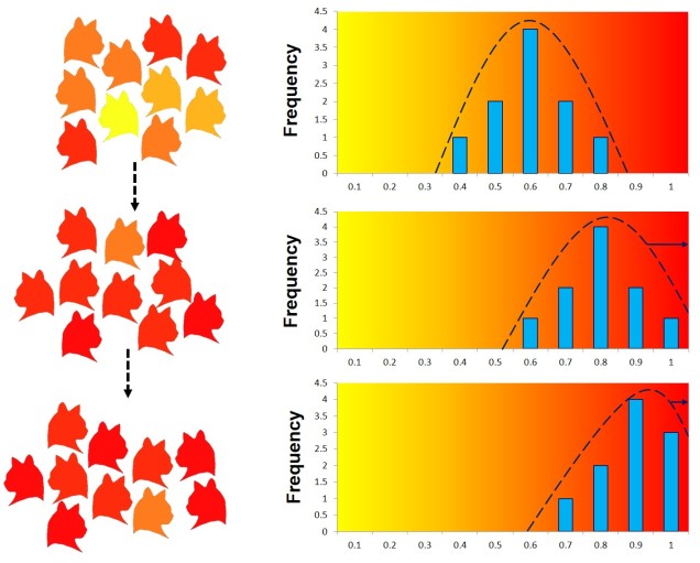
An example of directional selection. In this instance, we have one population of cats and a single phenotypic trait (colour) which ranges from 0 (yellow) to 1 (red). Red colour is selected for above all other colours; the original population has a pretty diverse mix of colours to start. Over time, we can see the average colour of the entire population moves towards more red colours whilst yellow colours start to disappear. Note that although the final population is predominantly red, there is still some (minor) variation in colours. These changes are reflected in the distribution of the colour-coding alleles (right), as it moves towards the red end of the spectrum.
Balancing selection
Natural selection doesn’t always push allele frequencies into different directions however, and sometimes maintains the diversity of alleles in the population. This is what happens in ‘balancing selection’ (sometimes also referred to as ‘stabilising selection’). In this example, natural selection favours non-extreme allele frequencies, and pushes the distribution of allele frequencies more to the centre. This may happen if deviations from the original gene, regardless of the specific change, can have strongly negative effects on the fitness of an organism, or in genes that are most fit when there is a decent amount of variation within them in the population (such as the MHC region, which contributes to immune response). There are a couple other reasons balancing selection may occur, though.
Heterozygote advantage
One example is known as ‘heterozygote advantage’. This is when an organism with two different alleles of a particular gene has greater fitness than an organism with two identical copies of either allele. A seemingly bizarre example of heterozygote advantage is related to sickle cell anaemia in African people. Sickle cell anaemia is a serious genetic disorder which is encoded for by recessive alleles of a haemoglobin gene; thus, a person has to carry two copies of the disease allele to show damaging symptoms. While this trait would ordinarily be strongly selected against in many population, it is maintained in some African populations by the presence of malaria. This seems counterintuitive; why does the presence of one disease maintain another?
Well, it turns out that malaria is not very good at infecting sickle cells; there are a few suggested mechanisms for why but no clear single answer. Naturally, suffering from either sickle cell anaemia or malaria is unlikely to convey fitness benefits. In this circumstance, natural selection actually favours having one sickle cell anaemia allele; while being a carrier isn’t ordinarily as healthy as having no sickle cell alleles, it does actually make the person somewhat resistant to malaria. Thus, in populations where there is a selective pressure from malaria, there is a heterozygote advantage for sickle cell anaemia. For those African populations without likely exposure to malaria, sickle cell anaemia is strongly selected against and less prevalent.
A diagram of how heterozygote advantage works in sickle cell anaemia and malaria resistance. On the top we have our two main traits: the blood cell shape (which has two different alleles; normal and sickle celled) and malaria infection by mosquitoes. Blue circles indicate that the trait has good fitness, whilst red crosses indicate the trait has bad fitness. For the left hand person, having two sickle cell alleles (ss) means they are symptomatic of sickle cell anaemia and is unlikely to have a good quality of life. On the right, having two normal blood cell alleles (SS) means that he is susceptible to malaria infection. The middle person, however, having only one sickle cell allele (Ss) means they are asymptomatic but still resistant to malaria. Thus, being heterozygous for sickle cell is actually beneficial over being homozygous in either direction: this is reflected in the distribution of alleles (bottom). The left side is pushed down by sickle cell anaemia whilst the right side is pushed down by malaria, thus causing both blood cell alleles (s and S) to be maintained at an intermediate frequency (i.e. balanced).
Frequency-dependent selection
Another form of balancing selection is called ‘frequency-dependent selection’, where the fitness of an allele is inversely proportional to its frequency. Thus, once the allele has become common due to selection, the fitness of that allele is reduced and selection will start to favour the alternative allele (which is at much lower frequency). The constant back-and-forth tipping of the selective scales results in both alleles being maintained at an equilibrium.
This can happen in a number of different ways, but often the rarer trait/allele is fundamentally more fit because of its rarity. For example, if one allele allows an individual to use a new food source, it will be very selectively fit due to the lack of competition with others. However, as that allele accumulates within the population and more individuals start to feed on that food source, the lack of ‘uniqueness’ will mean that it’s not particularly better than the original food source. A balance between the two food sources (and thus alleles) will be maintained over time as shifts towards one will make the other more fit, and natural selection will compensate.
An example of frequency-dependent selection. The colour of the cat indicates both their genotype and their food sources: black cats eat red apples whilst green cats eat green apples (this species has apparently developed herbivory, okay?) To start with, the incredibly low frequency of green cats mean that the one green cat can exploit a huge food source compared to black cats. Because of this, natural selection favours green cats. However, in the next generation evolution overcompensates and produces way too many green cats, and now black cats are getting much more food. Natural selection bounces back to favour black cats. Eventually, this causes and equilibrium balance of the two cat types (as shifts one way will cause a shift back the other way immediately after). These changes are reflected in the overall frequency of the two types over time (top right), which eventually evens out. The bottom right figure demonstrates that for both cat types, the frequency of that colour is inversely proportional to the overall fitness (measured as a proxy by amount of food per cat).
Disruptive selection
A third category of selection (although not as frequently mentioned) is known as ‘disruptive selection’, which is essentially the direct opposite of balancing selection. In this case, both extremes of allele frequencies are favoured (e.g. 1 for one allele or 1 for the other) but intermediate frequencies are not. This can be difficult to untangle in natural populations since it could technically be attributed to two different cases of directional selection. Each allele of the same gene is directionally selected for, but in opposite populations and directions so that overall pattern shows very little intermediates.
In direct contrast to balancing selection, disruptive selection can often be a case of heterozygote disadvantage (although it’s rarely called that). In these examples, it may be that individuals which are not genetically committed to one end or the other of the frequency spectrum are maladapted since they don’t fit in anywhere. An example would be a species that occupies both the desert and a forested area, with little grassland-type habitat in the middle. For the relevant traits, strongly desert-adapted genes would be selected for in the desert and strongly forest-adapted genes would be selected for in the forest. However, the lack of gradient between the two habitats means that individuals that are half-and-half are less adaptive in both the desert and the forest. A case of jack-of-all-trades, master of none.
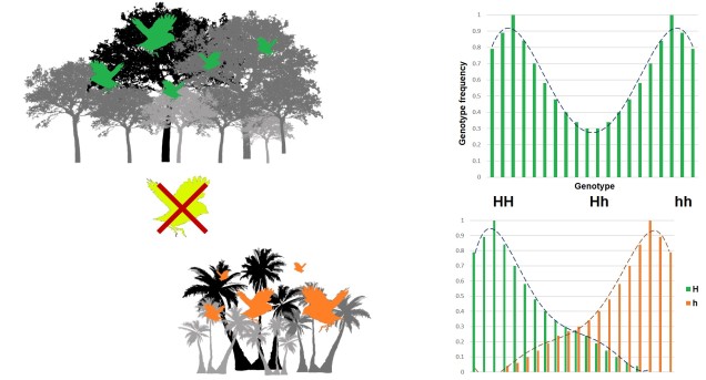
The above example of disruptive selection. Bird colour is coded for by a single gene; green birds have a HH genotype, orange birds have a hh genotype, and yellow birds are heterozygotes (Hh). Habitats where the two homozygote colours are most adaptive are found; green birds do well in the forest whereas orange birds do well in the desert. However, there’s no intermediate habitat between the two and so yellow birds don’t really fit well anywhere; they’re outcompeted in the forest and desert by the respective other colours. This means selection favours either extreme (homozygotes), shown in the top right. If we split up the two alleles of the genotype though, we can see that this disruptive selection is really the product of two directionally selective traits working in inverse directions: H is favoured at one end and h at the other.
Direction of selection
Although it would be convenient if natural selection was entirely predictable, it often catches up by surprise in how it acts and changes species and populations in the wild. Careful analysis and understanding of the different processes and outcomes of adaptation can feed our overall understanding of evolution, and aid in at least pointing in the right direction for our predictions.
The phrase ‘fake news’ seems to get thrown around ad nauseum these days, but there’s a reason for it (besides the original somewhat famous coining of the phrase). Inadvertently bad, or sometimes downright malicious, reporting of various apparent ‘trends’ or ‘patterns’ are rife throughout nearly all forms of media. Particularly, many entirely subjective or blatantly falsified presentations or reports of ‘fact’ cloud real scientific inquiry and its distillation into the broader community. In fact, a recent study has shown that falsified science spreads through social media at orders of magnitude faster than real science: so why is this? And how do we spot the real from the fake?
It’s imperative that we understand what real science entails to be able to separate it from the pseudoscience. Of course, scientific rigour and method are always of utmost importance, but these can be hard to detect (or can be effectively lied through colourful language choices). When reading a scientific article, whether it’s direct from the source (a journal, such as Nature or Science) or secondarily through a media outlet such as the news or online sources, there’s a few things that you should always look for that will help discern between the two categories.
Peer-review and adequate referencing
Firstly, is the science presented in an objective, logical manner? Does it systematically demonstrate the study system and question, with the relevant reference to peer-reviewed literature? Good science builds upon the wealth of previously done good science to contribute to a broader field of knowledge; in this way, critical observations and alternative ideas can be compared and contrasted to steer the broader field. Even entirely novel science, which go against the common consensus, will reference and build upon prior literature and justify the necessity and design of the study. Having written more than one literature review in my life, I can safely assure you that there is no shortage of relevant scientific studies that need to be read, understood and built upon in any future scientific study.
Methods, statistics and sampling
Secondly, is there a solid methodological basis for the science? In almost all cases this will include some kind of statistical measure for the validity (and accuracy) of the results. How does the sample size of the study measure up to what the target group? Remember, a study size of 500 people is definitely too small to infer the medical conditions of all humans, but rarely do we get sample sizes that big in evolutionary genetics studies (especially in non-model species). The sampling regime is extremely important for interpreting the results: particularly, keep in mind if there is an inherent bias in the way the sampling has been done. Are some groups more represented than others? Where do the samples come from? What other factors might be influencing the results, based on the origin of the samples?
Despite having a large sample size, and a significant result (p<0.05), this study cannot conclude that all dogs are awful. It can conclude, however, that cats are statistically significant assholes.
Presentation and language of findings
Thirdly, how does the source present the results? Does it make claims that seem beyond a feasible conclusion based on the study itself? Even if the underlying study is scientific, many secondary sources have a tendency to ‘sensationalise’ the results in order to make them both more appealing and more digestible to the general public. This is only exacerbated by the lack of information of the scientific method of the original paper, actual statistics, or the accurate summation of those statistics. Furthermore, a real scientific study will try to (in most cases) avoid evocative words such as ‘prove’, as a fundamental aspect of science is that no study is 100% ‘proven’ (see falsifiability below). Proofs are a relevant mathematical concept though, but these fall under a different category altogether.
Here’s an example: recently, an Australian mainstream media outlet (among many) shared a story about a ‘recent’ (six months old) study that found that second-born children are more likely to be criminals and first-born children have higher IQ. As you might expect, the original studydoes not imply that being born second will make you a sudden murderer nor will being the first born make you a prodigy. Instead, the authors suggest that there may be a link between differential parental investment/attention (between different age order children) as a potential mechanism. They ruled out, based on a wealth of statistics, the influence of alternative factors such as health or education (both in quality and quantity). Thus, there is a correlative (read: not causative) effect of age on these characteristics. If you directly interpreted the newscast (or read some of the misguided comments), you might think otherwise.
Falsifiability
Fourthly, are the hypotheses in the study falsifiable? One of the foundations of the modern scientific method includes the requirement of any real scientific hypothesis to be falsifiable; that is, there must be a way to show evidence against that hypothesis. This can be difficult to evaluate, but is why some broad philosophical questions are considered ‘unscientific’. A classic example is the phrase “all swans are white”, which was apparently historically believed in Europe (where there are no black swans). This statement is technically falsifiable, since if one found a non-white swan it would ‘disprove’ the hypothesis. Lo and behold, Europeans arrive in Australia and find that, actually, some swans are black. The original statement was thus falsified.
Well, I’ll be damned falsified. Just pretend the swan is actually black: I don’t have enough ink to make it realistic…
The role of the peer: including you!
Peer-review is a critical aspect of scientific process, and despite some conspiracy-theory-esque remarks about the secret Big Science Society, it generally works. While independent people inevitably have their own personal biases and are naturally subjective to some degree (no matter how hard we may try to be objective), a larger number of well-informed, critical thinkers help to broaden the focus and perspective surrounding any scientific subject. Remember, nothing is more critical of science than science itself.
One of the most apt representations of peer-review I’ve ever seen, from Dr. Nick D. Kim (PhD). Source: here.
While peer-review is technically aimed at other scientists as a way to steer and inform research, the input of outsider, non-specialist readers can still be informative. By closely looking at science, and better understanding both how it is done and what it is showing, can help us evaluate how valuable science is to broader society and shift scientific information into useful, everyday applications. Furthermore, by educating ourselves on what is real science, and what is disruptive drivel, we can aid the development of science and reduce the slowing impact of misinformation and deceit.