The many genetic faces of adaptation

The transition from genotype to phenotype

While evolutionary genetics studies often focus on the underlying genetic architecture of species and populations to understand their evolution, we know that natural selection acts directly on physical characteristics. We call these the phenotype; by studying changes in the genes that determine these traits (the genotype), we can take a nuanced approach at studying adaptation. However, our ability to look at genetic changes and relate these to a clear phenotypic trait, and how and why that trait is under natural selection, can be a difficult task.

One gene for one trait

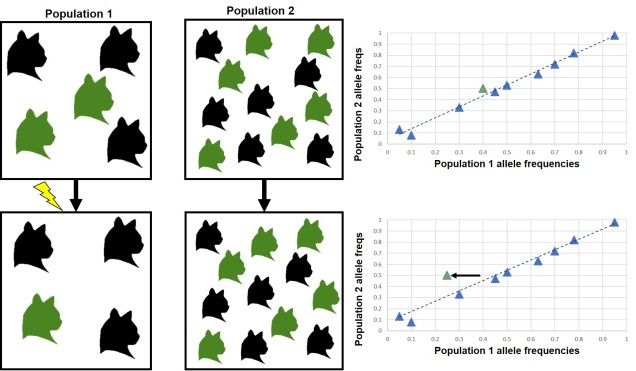
The simplest (and most widely used) models of understanding the genetic basis of adaptation assume that a single genotype codes for a single phenotypic trait. This means that changes in a single gene (such as outliers that we have identified in our analyses) create changes in a particular physical trait that is under a selective pressure in the environment. This is a useful model because it is statistically tractable to be able to identify few specific genes of very large effect within our genomic datasets and directly relate these to a trait: adding more complexity exponentially increases the difficulty in detecting patterns (at both the genotypic and phenotypic level).

Single locus figure
An example of a single gene coding for a single phenotypic trait. In this example, the different combination of alleles of the one gene determines the colour of the cat.

Many genes for one trait: polygenic adaptation

Unfortunately, nature is not always convenient and recent findings suggest that the overwhelming majority of the genetics of adaptation operate under what is called ‘polygenic adaptation’. As the name suggestions, under this scenario changes (even very small ones) in many different genes combine together to have a large effect on a particular phenotypic trait. Given the often very small magnitude of the genetic changes, it can be extremely difficult to separate adaptive changes in genes from neutral changes due to genetic drift. Likewise, trying to understand how these different genes all combine into a single functional trait is almost impossible, especially for non-model species.

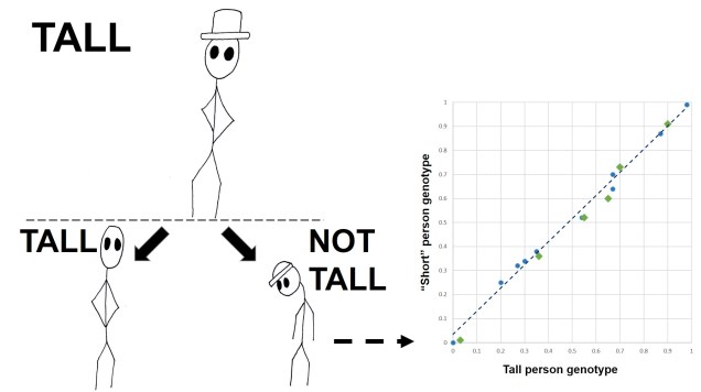
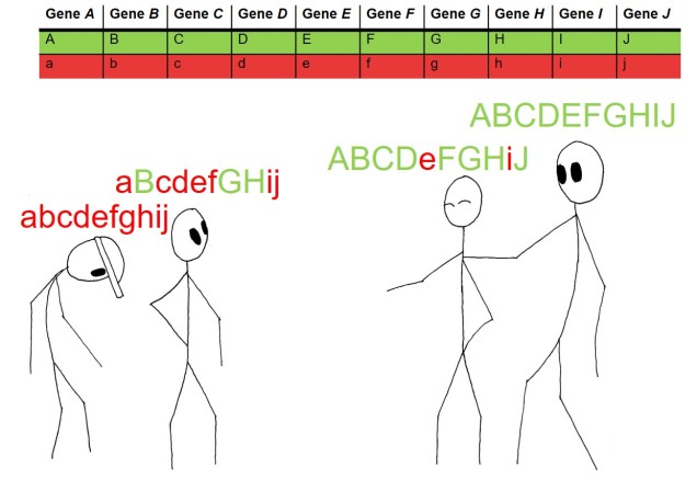
Polygenic adaptation is often seen for traits which are clearly heritable, but don’t show a single underlying gene responsible. Previously, we’ve covered this with the heritability of height: this is one of many examples of ‘quantitative trait loci’ (QTLs). Changes in one QTL (a single gene) causes a small quantitative change in a particular trait; the combined effect of different QTLs together can ‘add up’ (or counteract one another) to result in the final phenotype value.

Height QTL
An example of polygenic quantitative trait loci. In this example, height is partially coded for by a total of ten different genes: the dominant form of each gene (Capitals, green) provides more height whereas the recessive form (lowercase, red) doesn’t. The cumulative total of these components determines how tall the person is: the person on the far right was very unlucky and got 0/10 height bonuses and so is the shortest. Progressively from left to right, some genes are contributing to the taller height of the people, with the far right person standing tall with the ultimate 10/10 pro-height genes. For reference, height is actually likely to be coded for by thousands of genes, not 10.

The mechanisms which underlie polygenic adaptation can be more complex than simple addition, too. Individual genes might cause phenotypic changes which interact with other phenotypes (and their underlying genotypes) to create a network of changes. We call these interactions ‘epistasis’, where changes in one gene can cause a flow-on effect of changes in other genes based on how their resultant phenotypes interact. We can see this in metabolic pathways: given that a series of proteins are often used in succession within pathways, a change in any single protein in the process could affect every other protein in the pathway. Of course, knowing the exact proteins coded for every gene, including their physical structure, and how each of those proteins could interact with other proteins is an immense task. Similar to QTLs, this is usually limited to model species which have a large history of research on these specific areas to back up the study. However, some molecular ecology studies are starting to dive into this area by identifying pathways that are under selection instead of individual genes, to give a broader picture of the overall traits that are underlying adaptation.

Labrador epistasis figure
My favourite example of epistasis on coat colour in labradors. Two genes together determine the colour of the coat, with strong interactions between them. The first gene (E/e) determines whether or not the underlying coat gene (B/b) is masked or not: two recessive alleles of the first gene (ee) completely blocks Gene 2 and causes the coat to become golden regardless of the second gene genotype (much like my beloved late childhood pet pictured, Sunny). If the first gene has at least one dominant allele, then the second gene is allowed to express itself. Possessing a dominant allele (BB or Bb) leads to a black lab; possessing two recessive alleles (bb) makes a choc lab!
Labrador epistasis table
The possible combinations of genotypes for the two above genes and the resultant coat colour (indicated by the box colour).

One gene for many traits: pleiotropy and differential gene expression

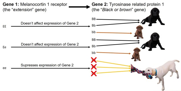
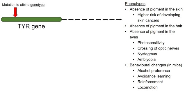
In contrast to polygenic traits, changes in a single gene can also potentially alter multiple phenotypic traits simultaneously. This is referred to as ‘pleiotropy’ and can happen if a gene has multiple different functions within an organism; one particular protein might be a component of several different systems depending on where it is found or how it is arranged. A clear example of pleiotropy is in albino animals: the most common form of albinism is the result of possessing two recessive alleles of a single gene (TYR). The result of this is the absence of the enzyme tyrosinase in the organism, a critical component in the production of melanin. The flow-on phenotypic effects from the recessive gene most obviously cause a lack of pigmentation of the skin (whitening) and eyes (which appear pink), but also other physiological changes such as light sensitivity or total blindness (due to changes in the iris). Albinism has even been attributed to behavioural changes in wild field mice.

Albinism pleiotropy
A very simplified diagram of how one genotype (the albino version of the TYR gene) can lead to a large number of phenotypic changes via pleiotropy (although many are naturally physiologically connected).

Because pleiotropic genes code for several different phenotypic traits, natural selection can be a little more complicated. If some resultant traits are selected against, but others are selected for, it can be difficult for evolution to ‘resolve’ the balance between the two. The overall fitness of the gene is thus dependent on the balance of positive and negative fitness of the different traits, which will determine whether the gene is positively or negatively selected (much like a cost-benefit scenario). Alternatively, some traits which are selectively neutral (i.e. don’t directly provide fitness benefits) may be indirectly selected for if another phenotype of the same underlying gene is selected for.

Multiple phenotypes from a single ‘gene’ can also arise by alternate splicing: when a gene is transcribed from the DNA sequence into the protein, the non-coding intron sections within the gene are removed. However, exactly which introns are removed and how the different coding exons are arranged in the final protein sequence can give rise to multiple different protein structures, each with potentially different functions. Thus, a single overarching gene can lead to many different functional proteins. The role of alternate splicing in adaptation and evolution is a rarely explored area of research and its importance is relatively unknown.

Non-genes for traits: epigenetics

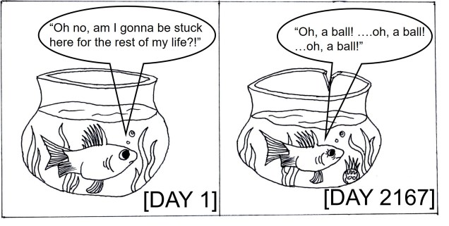
This gets more complicated if we consider ‘non-genetic’ aspects underlying the phenotype in what we call ‘epigenetics’. The phrase literally translates as ‘on top of genes’ and refers to chemical attachments to the DNA which control the expression of genes by allowing or resisting the transcription process. Epigenetics is a relatively new area of research, although studies have started to delve into the role of epigenetic changes in facilitating adaptation and evolution. Although epigenetics is still a relatively new research topic, future research into the relationship between epigenetic changes and adaptive potential might provide more detailed insight into how adaptation occurs in the wild (and might provide a mechanism for adaptation for species with low genetic diversity)!


The different interactions between genotypes, phenotypes and fitness, as well as their complex potential outcomes, inevitably complicates any study of evolution. However, these are important aspects of the adaptation process and to discard them as irrelevant will not doubt reduce our ability to examine and determine evolutionary processes in the wild.

Fantastic Genes and Where to Find Them

The genetics of adaptation

Adaptation and evolution by natural selection remains one of the most significant research questions in many disciplines of biology, and this is undoubtedly true for molecular ecology. While traditional evolutionary studies have been based on the physiological aspects of organisms and how this relates to their evolution, such as how these traits improve their fitness, the genetic component of adaptation is still somewhat elusive for many species and traits.

Hunting for adaptive genes in the genome

We’ve previously looked at the two main categories of genetic variation: neutral and adaptive. Although we’ve focused predominantly on the neutral components of the genome, and the types of questions about demographic history, geographic influences and the effect of genetic drift, they cannot tell us (directly) about the process of adaptation and natural selective changes in species. To look at this area, we’d have to focus on adaptive variation instead; that is, genes (or other related genetic markers) which directly influence the ability of a species to adapt and evolve. These are directly under natural selection, either positively (‘selected for’) or negatively (‘selected against’).

Given how complex organisms, the environment and genomes can be, it can be difficult to determine exactly what is a real (i.e. strong) selective pressure, how this is influenced by the physical characteristics of the organism (the ‘phenotype’) and which genes are fundamental to the process (the ‘genotype’). Even determining the relevant genes can be difficult; how do we find the needle-like adaptive genes in a genomic haystack?

Magnifying glass figure
If only it were this easy.

There’s a variety of different methods we can use to find adaptive genetic variation, each with particular drawbacks and strengths. Many of these are based on tests of the frequency of alleles, rather than on the exact genetic changes themselves; adaptation works more often by favouring one variant over another rather than completely removing the less-adaptive variant (this would be called ‘fixation’). So measuring the frequency of different alleles is a central component of many analyses.

FST outlier tests

One of the most classical examples is called an ‘FST outlier test’. This can be a bit complicated without understanding what FST is actually measures: in short terms, it’s a statistical measure of ‘population differentiation due to genetic structure’. The FST value of one particular population can determine how genetically similar it is to another. An FST value of 1 implies that the two populations are as genetically different as they could possibly be, whilst an FST value of 0 implies that they are genetically identical populations.

Generally, FST reflects neutral genetic structure: it gives a background of how, on average, different are two populations. However, if we know what the average amount of genetic differentiation should be for a neutral DNA marker, then we would predict that adaptive markers are significantly different. This is because a gene under selection should be more directly pushed towards or away from one variant (allele) than another, and much more strongly than the neutral variation would predict. Thus, the alleles that are way more or less frequent than the average pattern we might assume are under selection. This is the basis of the FST outlier test; by comparing two or more populations (using FST), and looking at the distribution of allele frequencies, we can pick out a few alleles that vary from the average pattern and suggest that they are under selection (i.e. are adaptive).

There are a few significant drawbacks for FST outlier tests. One of the most major ones is that genetic drift can also produce a large number of outliers; in a small population, for example, one allele might be fixed (has a frequency of 1, with no alternative allele in the population) simply because there is not enough diversity or population size to sustain more alleles. Even if this particular allele was extremely detrimental, it’d still appear to be favoured by natural selection just because of drift.

Drift leading to outliers diagram
An example of genetic drift leading to outliers, featuring our friends the cat population. Top row: Two cat populations, one small (left; n = 5) and one large (middle, n = 12) show little genetic differentiation between them (right; each triangle represents a single gene or locus; the ‘colour’ gene is marked in green). The average (‘neutral’) pattern of differentiation is shown by the dashed line. Much like in our original example, one cat in the small population is horrifically struck by lightning and dies (RIP again). Now when we compare the frequency of the alleles of the two populations (bottom), we see that (because a green cat died), the ‘colour’ locus has shifted away from the general trend (right) and is now an outlier. Thus, genetic drift in the ‘colour’ gene gives the illusion of a selective loci (even though natural selection didn’t cause the change, since colour does not relate to how likely a cat is to be struck by lightning).

Secondly, the cut-off for a ‘significant’ vs. ‘relatively different but possibly not under selection’ can be a bit arbitrary; some genes that are under weak selection can go undetected. Furthermore, recent studies have shown a growing appreciation for polygenic adaptation, where tiny changes in allele frequencies of many different genes combine together to cause strong evolutionary changes. For example, despite the clear heritable nature of height (tall people often have tall children), there is no clear ‘height’ gene: instead, it appears that hundreds of genes are potentially very minor height contributors.

Polygenic height figure final
In this example, we have one tall parent (top) who produces two offspring; one who is tall (left) and one who isn’t (right). In order to understand what genetic factors are contributing to their height differences, we compare their genetics (right; each dot represents a single locus). Although there aren’t any particular loci that look massively different between the two, the cumulative effect of tiny differences (the green triangles) together make one person taller than the other. There are no clear outliers, but many (poly) different genes (genic) acting together.

Genotype-environment associations

To overcome these biases, sometimes we might take a more methodological approach called ‘genotype-environment association’. This analysis differs in that we select what we think our selective pressures are: often environmental characteristics such as rainfall, temperature, habitat type or altitude. We then take two types of measures per individual organism: the genotype, through DNA sequencing, and the relevant environmental values for that organisms’ location. We repeat this over the full distribution of the species, taking a good number of samples per population and making sure we capture the full variation in the environment. Then we perform a correlation-type analysis, which seeks to see if there’s a connection or trend between any particular alleles and any environmental variables. The most relevant variables are often pulled out of the environmental dataset and focused on to reduce noise in the data.

The main benefit of GEA over FST outlier tests is that it’s unlikely to be as strongly influenced by genetic drift. Unless (coincidentally) populations are drifting at the same genes in the same pattern as the environment, the analysis is unlikely to falsely pick it up. However, it can still be confounded by neutral population structure; if one population randomly has a lot of unique alleles or variation, and also occurs in a somewhat unique environment, it can bias the correlation. Furthermore, GEA is limited by the accuracy and relevance of the environmental variables chosen; if we pick only a few, or miss the most important ones for the species, we won’t be able to detect a large number of very relevant (and likely very selective) genes. This is a universal problem in model-based approaches and not just limited to GEA analysis.

New spells to find adaptive genes?

It seems likely that with increasing datasets and better analytical platforms, many more types of analysis will be developed to delve deeper into the adaptive aspects of the genome. With whole-genome sequencing starting to become a reality for non-model species, better annotation of current genomes and a steadily increasing database of functional genes, the ability of researchers to investigate evolution and adaptation at the genomic level is also increasing.

Evolution and the space-time continuum

Evolution travelling in time

As I’ve mentioned a few times before, evolution is a constant force that changes and flows over time. While sometimes it’s more convenient to think of evolution as a series of rather discrete events (a species pops up here, a population separates here, etc.), it’s really a more continual process. The context and strength of evolutionary forces, such as natural selection, changes as species and the environment they inhabit also changes. This is important to remember in evolutionary studies because although we might think of more recent and immediate causes of the evolutionary changes we see, they might actually reflect much more historic patterns. For example, extremely low contemporary levels of genetic diversity in cheetah is likely largely due to a severe reduction in their numbers during the last ice age, ~12 thousand years ago (that’s not to say that modern human issues haven’t also been seriously detrimental to them). Similarly, we can see how the low genetic diversity of a small population colonise a new area can have long term effects on their genetic variation: this is called ‘founder effect’. Because of this, we often have to consider the temporal aspect of a species’ evolution.

Founder effect diagram
An example of founder effect. Each circle represents a single organism; the different colours are an indicator of how much genetic diversity that individual possesses (more colours = more variation). We start with a single population; one (A) or two (B) individuals go on a vacation and decide to stay on a new island. Even after the population has become established and grows over time, it takes a long time for new diversity to arise. This is because of the small original population size and genetic diversity; this is called founder effect. The more genetic diversity in the settled population (e.g. vs A), the faster new diversity arises and the weaker the founder effect.

Evolution travelling across space

If the environmental context of species and populations are also important for determining the evolutionary pathways of organisms, then we must also consider the spatial context. Because of this, we also need to look at where evolution is happening in the world; what kinds of geographic, climatic, hydrological or geological patterns are shaping and influencing the evolution of species? These patterns can influence both neutral or adaptive processes by shaping exactly how populations or species exist in nature; how connected they are, how many populations they can sustain, how large those populations can sustainably become, and what kinds of selective pressures those populations are under.

Allopatry diagram
An example of how the environment (in this case, geology) can have both neutral and adaptive effects. Let’s say we start with one big population of cats (N = 9; A), which is distributed over a single large area (the green box). However, a sudden geological event causes a mountain range to uplift, splitting the population in two (B). Because of the reduced population size and the (likely) randomness of which individuals are on each side, we expect some impact of genetic drift. Thus, this is the neutral influence. Over time, these two separated regions might change climatically (C), with one becoming much more arid and dry (right) and the other more wet and shady (left). Because of the difference of the selective environment, the two populations might adapt differently. This is the adaptive influence. 

Evolution along the space-time continuum

Given that the environment also changes over time (and can be very rapid, and we’ve seen recently), the interaction of the spatial and temporal aspects of evolution are critical in understanding the true evolutionary history of species. As we know, the selective environment is what determines what is, and isn’t, adaptive (or maladaptive), so we can easily imagine how a change in the environment could push changes in species. Even from a neutral perspective, geography is important to consider since it can directly determine which populations are or aren’t connected, how many populations there are in total or how big populations can sustainably get. It’s always important to consider how evolution travels along the space-time continuum.

Genetics TARDIS
“Postgraduate Student Who” doesn’t quite have the same ring to it, unfortunately.

Phylogeography

The field of evolutionary science most concerned with these two factors and how the influence evolution is known as ‘phylogeography’, which I’ve briefly mentioned in previous posts. In essence, phylogeographers are interested in how the general environment (e.g. geology, hydrology, climate, etc) have influenced the distribution of genealogical lineages. That’s a bit of a mouthful and seems a bit complicated, by the genealogical part is important; phylogeography has a keen basis in evolutionary genetics theory and analysis, and explicitly uses genetic data to test patterns of historic evolution. Simply testing the association between broad species or populations, without the genetic background, and their environment, falls under the umbrella field of ‘biogeography’. Semantics, but important.

Birds phylogeo
Some example phylogeographic models created by Zamudio et al. (2016). For each model, there’s a demonstrated relationship between genealogical lineages (left) and the geographic patterns (right), with the colours of the birds indicating some trait (let’s pretend they’re actually super colourful, as birds are). As you can see, depending on which model you look at, you will see a different evolutionary pattern; for example, model shows specific lineages that are geographically isolated from one another each evolved their own colour. This contrasts with in that each colour appears to have evolved once in each region based on the genetic history.

For phylogeography, the genetic history of populations or species gives the more accurate overview of their history; it allows us to test when populations or species became separated, which were most closely related, and whether patterns are similar or different across other taxonomic groups. Predominantly, phylogeography is based on neutral genetic variation, as using adaptive variation can confound the patterns we are testing. Additionally, since neutral variation changes over time in a generally predictable, mathematical format (see this post to see what I mean), we can make testable models of various phylogeographic patterns and see how well our genetic data makes sense under each model. For example, we could make a couple different models of how many historic populations there were and see which one makes the most sense for our data (with a statistical basis, of course). This wouldn’t work with genes under selection since they (by their nature) wouldn’t fit a standard ‘neutral’ model.

Coalescent
If it looks mathematically complicated, it’s because it is. This is an example of the coalescent from Brito & Edwards, 2008: a method that maps genes back in time (the different lines) to see where the different variants meet at a common ancestor. These genes are nested within the history of the species as a whole (the ‘tubes’), with many different variables accounted for in the model.

That said, there are plenty of interesting scientific questions within phylogeography that look at exploring the adaptive variation of historic populations or species and how this has influenced their evolution. Although this can’t inherently be built into the same models as the neutral patterns, looking at candidate genes that we think are important for evolution and seeing how their distributions and patterns relate to the overall phylogeographic history of the species is one way of investigating historic adaptive evolution. For example, we might track changes in adaptive genes by seeing which populations have which variants of the gene and referring to our phylogeographic history to see how and when these variants arose. This can help us understand how phylogeographic patterns have influenced the adaptive evolution of different populations or species, or inversely, how adaptive traits might have influenced the geographic distribution of species or populations.

Where did you come from and where will you go?

Phylogeographic studies can tell us a lot about the history of a species, and particularly how that relates to the history of the Earth. All organisms share an intimate relationship with their environment, both over time and space, and keeping this in mind is key for understanding the true evolutionary history of life on Earth.


Drifting or driving: directionality in evolution

How random is evolution?

Often, we like to think of evolution fairly anthropomorphically; as if natural selection actively decides what is, and what isn’t, best for the evolution of a species (or population). Of course, there’s not some explicit Evolution God who decrees how a species should evolve, and in reality, evolution reflects a more probabilistic system. Traits that give a species a better chance of reproducing or surviving, and can be inherited by the offspring, will over time become more and more dominant within the species; contrastingly, traits that do the opposite will be ‘weeded out’ of the gene pool as maladaptive organisms die off or are outcompeted by more ‘fit’ individuals. The fitness value of a trait can be determined from how much the frequency of that trait varies over time.

So, if natural selection is just probabilistic, does this mean evolution is totally random? Is it just that traits are selected based on what just happens to survive and reproduce in nature, or are there more direct mechanisms involved? Well, it turns out both processes are important to some degree. But to get into it, we have to explain the difference between genetic drift and natural selection (we’re assuming here that our particular trait is genetically determined).  

Allele frequency over time diagram
The (statistical) overview of natural selection. In this example, we have two different traits in a population; the blue and the red O. Our starting population is 20 individuals (N), with 10 of each trait (a 1:1 ratio, or 50% frequency of each). We’re going to assume that, because the blue is favoured by natural selection, it doubles in frequency each generation (i.e. one individual with the blue has two offspring with one blue each). The red is neither here nor there and is stable over time (one red O produces one red O in the next generation). So, going from Gen 1 to Gen 2, we have twice as many blue Xs (Nt) as we did previously, changing the overall frequency of the traits (highlighted in yellow). Because populations probably don’t exponentially increase every generation, we’ll cut it back down to our original total of 20, but at the same ratios (Np). Over time, we can see that the population gradually accumulates more blue Xs relative to red Os, and by Gen 5 the red is extinct. Thus, the blue X has evolved!

When we consider the genetic variation within a species to be our focal trait, we can tell that different parts of the genome might be more related with natural selection than others. This makes sense; some mutations in the genome will directly change a trait (like fur colour) which might have a selective benefit or detriment, while others might not change anything physically or change traits that are neither here-nor-there under natural selection (like nose shape in people, for example). We can distinguish between these two by talking about adaptive or neutral variation; adaptive variation has a direct link to natural selection whilst neutral variation is predominantly the product of genetic drift. Depending on our research questions, we might focus on one type of variation over the other, but both are important components of evolution as a whole.

Genetic drift

Genetic drift is considered the random, selectively ‘neutral’ changes in the frequencies of different traits (alleles) over time, due to completely random effects such as random mutations or random loss of alleles. This results in the neutral variation we can observe in the gene pool of the species. Changes in allele frequencies can happen due to entirely stochastic events. If, by chance, all of the individuals with the blue fur variant of a gene are struck by lightning and die, the blue fur allele would end up with a frequency of 0 i.e. go extinct. That’s not to say the blue fur ‘predisposed’ the individuals to be struck be lightning (we assume here, anyway), so it’s not like it was ‘targeted against’ by natural selection (see the bottom figure for this example).

Because neutral variation appears under a totally random, probabilistic model, the mathematical basis of it (such as the rate at which mutations appear) has been well documented and is the foundation of many of the statistical aspects of molecular ecology. Much of our ability to detect which genes are under selection is by seeing how much the frequencies of alleles of that gene vary from the neutral model: if one allele is way more frequent than you’d expect by random genetic drift, then you’d say that it’s likely being ‘pushed’ by something: natural selection.

Manhattan plot example
A Manhattan plot, which measures the level of genetic differentiation between two different groups across the genome. The x-axis shows the length of the genome, in this example colour-coded by the specific chromosome of the sequence, while the y-axis shows the level of differentiation between the two groups being studied. The dots represent certain spots (loci, singular locus) in the genome, with the level of differentiation (Fst) measured for that locus in one group vs that locus in the other group. The dotted line represents the ‘average differentiation’: i.e. how different you’d expect the two groups to be by chance. Anything about that line is significantly different between the two groups, either because of drift or natural selection. This plot has been slightly adapted from Axelsson et al. (2013), who were studying domestication in dogs by comparing the genetic architecture of wild wolves versus domestic dogs. In this example we can see that certain regions of the genome are clearly different between dogs and wolves (circled); when the authors looked at the genes within those blocks, they found that many were related to behavioural changes (nervous system), competitive breeding (sperm-egg recognition) and interestingly, starch digestion. This last category suggests that adaptation to an omnivorous diet (likely human food waste) was key in the domestication process.

Natural selection

Contrastingly to genetic drift, natural selection is when particular traits are directly favoured (or unfavoured) in the environmental context of the population; natural selection is very specific to both the actual trait and how the trait works. A trait is only selected for if it conveys some kind of fitness benefit to the individual; in evolutionary genetics terms, this means it allows the individual to have more offspring or to survive better (usually).

While this might be true for a trait in a certain environment, in another it might be irrelevant or even have the reverse effect. Let’s again consider white fur as our trait under selection. In an arctic environment, white fur might be selected for because it helps the animal to camouflage against the snow to avoid predators or catch prey (and therefore increase survivability). However, in a dense rainforest, white fur would stand out starkly against the shadowy greenery of the foliage and thus make the animal a target, making it more likely to be taken by a predator or avoided by prey (thus decreasing survivability). Thus, fitness is very context-specific.

Who wins? Drift or selection?

So, which is mightier, the pen (drift) or the sword (selection)? Well, it depends on a large number of different factors such as mutation rate, the importance of the trait under selection, and even the size of the population. This last one might seem a little different to the other two, but it’s critically important to which process governs the evolution of the species.

In very small populations, we expect genetic drift to be the stronger process. Natural selection is often comparatively weaker because small populations have less genetic variation for it to act upon; there are less choices for gene variants that might be more beneficial than others. In severe cases, many of the traits are probably very maladaptive, but there’s just no better variant to be selected for; look at the plethora of physiological problems in the cheetah for some examples.

Genetic drift, however, doesn’t really care if there’s “good” or “bad” variation, since it’s totally random. That said, it tends to be stronger in smaller populations because a small, random change in the number or frequency of alleles can have a huge effect on the overall gene pool. Let’s say you have 5 cats in your species; they’re nearly extinct, and probably have very low genetic diversity. If one cat suddenly dies, you’ve lost 20% of your species (and up to that percentage of your genetic variation). However, if you had 500 cats in your species, and one died, you’d lose only <0.2% of your genetic variation and the gene pool would barely even notice. The same applies to random mutations, or if one unlucky cat doesn’t get to breed because it can’t find a mate, or any other random, non-selective reason. One way we can think of this is as ‘random error’ with evolution; even a perfectly adapted organism might not pass on its genes if it is really unlucky. A bigger sample size (i.e. more individuals) means this will have less impact on the total dataset (i.e. the species), though.

Drift in small pops
The effect of genetic drift on small populations. In this example, we have two very similar populations of cats, each with three different alleles (black, blue and green) in similar frequencies across the populations. The major difference is the size of the population; the left is much smaller (5 cats) compared to the right (20 cats). If one cat randomly dies from a bolt of lightning (RIP), and assuming that the colour of the cat has no effect on the likelihood of being struck by lightning (i.e. is not under natural selection), then the outcome of this event is entirely due to genetic drift. In this case, the left population has lost 1/5th of its population size and 1/3rd of its total genetic diversity thanks to the death of the genetically unique blue cat (He will be missed) whereas the right population has only really lost 1/20th of its size and no changes in total diversity (it’ll recover).

Both genetic drift and natural selection are important components of evolution, and together shape the overall patterns of evolution for any given species on the planet. The two processes can even feed into one another; random mutations (drift) might become the genetic basis of new selective traits (natural selection) if the environment changes to suit the new variation. Therefore, to ignore one in favour of the other would fail to capture the full breadth of the processes which ultimately shape and determine the evolution of all species on Earth, and thus the formation of the diversity of life.

“Who Do You Think You Are?”: studying the evolutionary history of species

The constancy of evolution

Evolution is a constant, endless force which seeks to push and shape species based on the context of their environment: sometimes rapidly, sometimes much more gradually. Although we often think of discrete points of evolution (when one species becomes two, when a particular trait evolves), it is nevertheless a continual force that influences changes in species. These changes are often difficult to ‘unevolve’ and have a certain ‘evolutionary inertia’ to them; because of these factors, it’s often critical to understand how a history of evolution has generated the organisms we see today.

What do I mean when I say evolutionary history? Well, the term is fairly diverse and can relate to the evolution of particular traits or types of traits, or the genetic variation and changes related to these changes. The types of questions and points of interest of evolutionary history can depend at which end of the timescale we look at: recent evolutionary histories, and the genetics related to them, will tell us different information to very ancient evolutionary histories. Let’s hop into our symbolic DeLorean and take a look back in time, shall we?

Labelled_evolhistory
A timeslice of evolutionary history (a pseudo-phylogenetic tree, I guess?), going from more recent history (bottom left) to deeper history (top right). Each region denoted in the tree represents the generally area of focus for each of the following blog headings. 1: Recent evolutionary history might look at individual pedigrees, or comparing populations of a single species. 2: Slightly older comparisons might focus on how species have arisen, and the factors that drive this (part of ‘phylogeography’). 3: Deep history might focus on the origin of whole groups of organisms and a focus on the evolution of particular traits like venom or sociality.

Very recent evolutionary history: pedigrees and populations

While we might ordinarily consider ‘evolutionary history’ to refer to events that happened thousands or millions of years ago, it can still be informative to look at history just a few generations ago. This often involves looking at pedigrees, such as in breeding programs, and trying to see how very short term and rapid evolution may have occurred; this can even include investigating how a particular breeding program might accidentally be causing the species to evolve to adapt to captivity! Rarely does this get referred to as true evolutionary history, but it fits on the spectrum, so I’m going to count it. We might also look at how current populations are evolving differently to one another, to try and predict how they’ll evolve into the future (and thus determine which ones are most at risk, which ones have critically important genetic diversity, and the overall survivability of the total species). This is the basis of ‘evolutionarily significant units’ or ESUs which we previously discussed on The G-CAT.

Captivefishcomic
Maybe goldfish evolved 3 second memory to adapt to the sheer boringness of captivity? …I’m joking, of course: the memory thing is a myth and adaptation works over generations, not a lifetime.

A little further back: phylogeography and species

A little further back, we might start to look at how different populations have formed or changed in semi-recent history (usually looking at the effect of human impacts: we’re really good at screwing things up I’m sorry to say). This can include looking at how populations have (or have not) adapted to new pressures, how stable populations have been over time, or whether new populations are being ‘made’ by recent barriers. At this level of populations and some (or incipient) species, we can find the field of ‘phylogeography’, which involves the study of how historic climate and geography have shaped the evolution of species or caused new species to evolve.

Evolution of salinity
An example of trait-based phylogenetics, looking at the biogeographic patterns and evolution/migration to freshwater in perch-like fishes, by Chen et al. (2014). The phylogeny shows that a group of fishes adapted to freshwater environments (black) from a (likely) saltwater ancestor (white), with euryhaline tolerance evolving two separate times (grey).

One high profile example of phylogeographic studies is the ‘Out of Africa’ hypothesis and debate for the origination of the modern human species. Although there has been no shortage of debate about the origin of modern humans, as well as the fate of our fellow Neanderthals and Denisovans, the ‘Out of Africa’ hypothesis still appears to be the most supported scenario.

human phylogeo
A generalised diagram of the ‘Out of Africa’ hypothesis of human migration, from Oppenheimer, 2012. 

Phylogeography is also component for determining and understanding ‘biodiversity hotspots’; that is, regions which have generated high levels of species diversity and contain many endemic species and populations, such as tropical hotspots or remote temperate regions. These are naturally of very high conservation value and contribute a huge amount to Earth’s biodiversity, ecological functions and potential for us to study evolution in action.

Deep, deep history: phylogenetics and the origin of species (groups)

Even further back, we start to delve into the more traditional concept of evolutionary history. We start to look at how species have formed; what factors caused them to become new species, how stable the new species are, and what are the genetic components underlying the change. This subfield of evolution is called ‘phylogenetics’, and relates to understanding how species or groups of species have evolved and are related to one another.

Sometimes, this includes trying to look at how particular diagnostic traits have evolved in a certain group, like venom within snakes or eusocial groups in bees. Phylogenetic methods are even used to try and predict which species of plants might create compounds which are medically valuable (like aspirin)! Similarly, we can try and predict how invasive a pest species may be based on their phylogenetic (how closely related the species are) and physiological traits in order to safeguard against groups of organisms that are likely to run rampant in new environments. It’s important to understand how and why these traits have evolved to get a good understanding of exactly how the diversity of life on Earth came about.

evolution of venom
An example of looking at trait evolution with phylogenetics, focusing on the evolution of venom in snakes, from Reyes-Velasco et al. (2014). The size of the boxes demonstrates the number of species in each group, with the colours reflecting the number of venomous (red) vs. non-venomous (grey) species. The red dot shows the likely origin of venom.

Phylogenetics also allows us to determine which species are the most ‘evolutionarily unique’; all the special little creatures of plant Earth which represent their own unique types of species, such as the tuatara or the platypus. Naturally, understanding exactly how precious and unique these species are suggests we should focus our conservation attention and particularly conserve them, since there’s nothing else in the world that even comes close!

Who cares what happened in the past right? Well, I do, and you should too! Evolution forms an important component of any conservation management plan, since we obviously want to make sure our species can survive into the future (i.e. adapt to new stressors). Trying to maintain the most ‘evolvable’ groups, particularly within breeding programs, can often be difficult when we have to balance inbreeding depression (not having enough genetic diversity) with outbreeding depression (obscuring good genetic diversity by adding bad genetic diversity into the gene pool). Often, we can best avoid these by identifying which populations are evolutionarily different to one another (see ESUs) and using that as a basis, since outbreeding vs. inbreeding depression can be very difficult to measure. This all goes back to the concept of ‘adaptive potential’ that we’ve discussed a few times before.

In any case, a keen understanding of the evolutionary trajectory of a species is a crucial component for conservation management and to figure out the processes and outcomes of evolution in the real world. Thus, evolutionary history remains a key area of research for both conservation and evolution-related studies.