As we discussed in last week’s post, different parts of the DNA can be used as genetic markers for analyses relating to conservation, ecology and evolution. We looked at a few different types of markers (allozymes, microsatellites, mitochondrial DNA) and why different markers are good for different things. This week, we’ll focus on the much grander and more modern state of genomics; that is, using DNA markers that are often thousands of genes big!
If we pretended that the size of the text for each marker was indicative of how big the data is, this figure would probably be about a 1000x under-estimationof genomic datasets. There is not enough room on the blog page to actually capture this.
I briefly mentioned last week that the development of genomics was largely facilitated by what we call ‘next-generation sequencing’, which allows us to easily obtain billions of fragments of DNA and collate them into a useful dataset. Most genomic technologies differ based on how they fragment the DNA for sequencing and how the data is processed.
While the analytical, monetary and time cost of obtaining genomic data has decreased as sequencing technology has improved, we still need to balance these factors together when deciding which method to use. Many methods allow us to put many individual samples together in the same reaction (we tell which sequence belongs to which sequence using special ‘barcode sequences’ that code for one specific sample): in this case, we also need to consider how many samples to place together (“multiplex”).
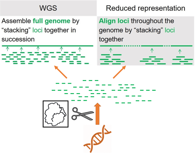
As a broad generalisation, we can separate most genomic sequencing methods into two broad categories: whole genome or reduced-representation. As the name suggests, whole genome sequencing involves collecting the entire genome of the individuals we use, although this is generally very expensive and can only be done with a limited number of samples at a time. If we want to have a much larger dataset, often we’ll use reduced-representation methods: these involve breaking down the whole genome into much smaller fragments and as many of these as we can to get a broad overview of the genome. Reduced-representation methods are much cheaper and are appropriate for larger sample sizes than whole genome, but naturally lose large amounts of information from the genome.
The (very, very) vague outline of genomic sequencing. First we take all of the DNA of an organism, breaking it into smaller fragments in this case using a restriction enzyme (see below). We then amplify these fragments, making billions of copies of them before piecing them back together to either make the entire genome (left) of a few individuals or patches of the genome (right) for more individuals.
Restriction-site associated DNA (RADseq)
Within the Molecular Ecology Lab, we predominantly use a technology known as “double digest restriction site-associated DNA sequencing”, which is a huge mouthful so we just call it ‘ddRAD’. This sounds incredibly complicated, but (as far as sequencing methods go, anyway) is actually relatively simple. We take the genome of a sample, and then using particular enzymes (called ‘restriction enzymes’), we break the genome randomly down into small fragments (usually up to 200 bases long, after we filter it). We then attach a specific barcode for that individual, and a few more bits and pieces as part of the sequencing process, and then pool them together. This pool (a “library”) is sent off to a facility to be run through a sequencing machine and produce the data we work with. The ‘dd’ part of ‘ddRAD’ just means that a pair of restriction enzymes are used in this method, instead of just one (it’s a lot cleaner and more efficient).
A simplified standard ddRAD protocol. 1) We obtain the DNA-containing tissue of the organism we want to study, such as blood, skin or muscle samples. 2) We extract all of the genomic DNA from the tissue sample, making sure we have good quantity and quality (avoiding degradation if possible). 3) We break the genome down into smaller fragments using restriction enzymes, which cut at certain places (orange and green marks on the top line). We then attach special sequences to these fragments, such as the adapter (needed for the sequencer to work) and the barcode for that specific individual organism (the green bar). 4) We amplify the fragments, generating billions of copies of each of them. 5) We send these off to a sequencing facility to read the DNA sequence of these fragments (often outsourced to a private institution). 6) We get back a massive file containing all of the different sequences for all of the organisms in one file. 7) We separate out these sequences into the individual the came from by using their special barcode as an identifier (the coloured codes). 8) We then process this data to make sure it’s of the best quality possible, including removing sequences that we don’t have enough copies of or have errors.From this, we produce a final dataset, often with one continuous sequence for each individual. If this dataset doesn’t meet our standards for quality or quantity, we go back and try new filtering parameters.
Gene expression and transcriptomics
Sometimes, however, we might not even want to look at the exact DNA sequence. You might remember in an earlier blog post that I mentioned genes can be ‘switched on’ or ‘switched off’ by activator or repressor proteins. Well, because of this, we can have the exact same genes act in different ways depending on the environment. This is most observable in tissue development: although all of the cells of all of your organs have the exact same genome, the control of gene expression changes what genes are active and thus the physiology of the organ. We might also have genes which are only active in an organism under certain conditions, like heat shock proteins under hot conditions.
This can be an important part of evolution as being able to easily change genetic expression may allow an individual to adapt to new environmental pressures much more easily; we call this ‘phenotypic plasticity’. In this case, instead of sequencing the DNA, we might want to look at which genes are expressed, or how much they are expressed, in different conditions or populations: this is called ‘comparative transcriptomics’. So instead of sequencing the DNA, we sequence the RNA of an organism (the middle step of making proteins, so most RNAs are only present if the gene is being expressed).
Processing data
Despite how it must appear, most of the work with genomic datasets actually comes after you get the sequences back. Because of the nature and scale of genomic datasets, rigorous analytical pipelines are needed to manage and filter data from the billions of small sequences into full sequences of high quality. There are many different ways to do this, and usually involves playing with parameters, so I won’t delve into the details (although some of it is explained in the boxed part of the flowchart figure).
The future of genomics
No doubt as the technology improves, whole genome sequencing will become progressively more feasible for more species, opening up the doors for a new avalanche of data and possibilities. In any case, we’ve come a long way since the first whole genome (for Haemophilus influenzae) in 1995 and the construction of the whole humangenome in 2003.
As we’ve previously discussed within The G-CAT, information from the DNA of organisms can be used in a variety of ways to study evolution and ecology, inform conservation management, and understand the diversity of life on Earth. We’ve also had a look at the general background of the DNA itself, and some of the different parts of the genome. What we haven’t discussed yet is how we use the DNA sequence in these studies; most importantly, which part of the genome to use.
The genome of most organisms is massive. The size of the genome ranges depending on the organism, with one of the smallest recorded genomes belonging to a bacteria (Carsonella ruddi), consisting of 160,000 bases. There is a bit of debate about the largest recorded genome, but one contender (the ‘canopy plant’, Paris japonica) has a genome stretching 150 billion base pairs long! The human genome sits in the middle at around 3 billion bases long. Naturally, it would be incredibly difficult to obtain the sequence of the whole genome of many organisms (particularly 20 – 30 years ago, due to technological limitations in the sequencing process) so instead we usually pick a specific region of the genome instead. The exact region (or type of region) we use is referred to as a ‘molecular marker’.
How do we choose a good marker?
The marker we pick is incredibly important: this is often based on how much variation we need to observe across groups. For example, if we want to study differences between individuals, say in a pedigree analysis, we need to pick a section of the DNA that will show differences between individuals; it will need to mutate fairly rapidly to be useful. If it mutates too slowly, all individuals will look identical genetically and we won’t have learnt anything new at all.
On the flipside, if we want to study evolution at a larger scale (say, between species, or groups of species) we would need to use a marker that evolves much slower. Using a rapidly mutating section of DNA would effectively give a tonne of ‘white noise’; it’d be impossible to pick what is the genetic difference at the species level (i.e. one species is different to another at that base) vs. at the individual level (i.e. one or many individuals within the species are different). Thus, we tend to use much slower mutating markers for deeper evolutionary history.
The spectrum of evolutionary history, with evolutionary splits between major animal groups on the left, to splits between species in the middle, to splits between individuals within a family tree on the right. The effectiveness of a marker for a particular part of the spectrum depends on its mutation rate. The original figure was taken from a landmark paper by Avise (1994), considered one of the forefathers of molecular ecology.
Think of it like comparing cats and dogs. If we wanted to compare different cats to one another (say different breeds) we could use hair length or coat colour as a useful trait. Since some breeds have different coat characteristics, and these don’t vary as much within the breed as across breeds, we can easily determine a long haired cat from a short haired cat. However, if we tried to use coat colour and length to compare cats and dogs we’d be stumped, because both species have lots of variation in these traits within their species. Some cats have coat length more similar to some dogs than to other cats for example; so they’re not a good characteristics to separate the two animal species (we might use muzzle shape, or body shape instead). If we substitute each of these traits with a particular marker, then we can see that some markers are better for some comparisons but not good for others.
Allozymes
The most traditional molecular marker are referred to as ‘allozymes’; instead of comparing actual genetic sequences (something that was not readily possible early in the field), variations in the shape (i.e. the amino acids of the protein, not the code underlying it) were compared between species. Changes in proteins occur very rarely as natural selection tends to push against randomly changing protein structure, since the shape of it is critical to its function and functionality. Because of this, allozymes were only really effective for studying very broad comparisons (mainly across species or species groups); the exact protein used depends on the study organism. Allozymes are generally considered outdated in the field nowadays.
With the development of technologies that allowed us to actual determine the DNA code of genes, molecular ecology moved into comparing actual sequences across individuals. However, early sequencing technology could generally only accurately determine small sections of DNA at a time, so particular markers capitalising on this were developed. Many of these are still used due to their cost-effectiveness and general ease of analysing.
Microsatellites
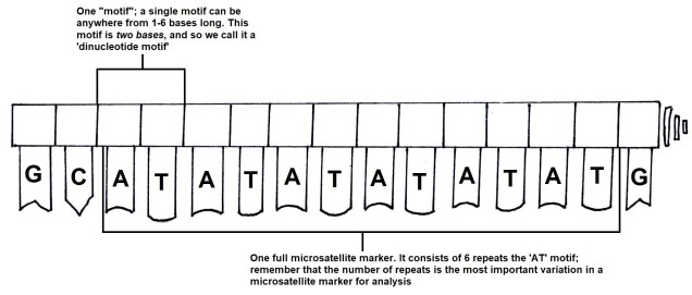
For comparing closely related individuals (within a pedigree, or a population), markers called ‘microsatellites’ are widely used. These are small sections of the genome which have repetitive DNA codes; usually, the same two or three base pairs (one ‘motif’) are repeated a number of times afterwards (the ‘repeat number’). While the motifs themselves rarely get mutations, the number of repeated motifs very rapidly mutates. This is because the protein that copies DNA is not very perfect, and often ‘slips up’, and adds or cuts off a repeat from the microsatellite sequence. Thus, differences in the repeat number of microsatellites accumulate pretty quickly, to the point where you can determine the parents of an individual with them.
The general (and simplified) structure of a microsatellite marker.
Microsatellites are often used in comparisons across closely related individuals, such as within pedigrees or within populations. While they are relatively easy to obtain, one drawback is that you need to have some understanding of the exact microsatellite you wish to analyse before you start; you need to make a specific ‘primer’ sequence to be able to get the right marker, as some may not be informative in particular species or comparisons. Many researchers choose to use 10-20 different microsatellite markers together in these types of studies, such as in human parentage analyses.
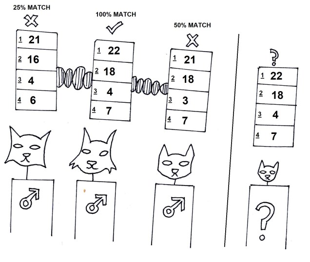
Microsatellites are useful for parentage analysis. Our previous guest contestants are here to discuss ‘Who is the father?!’ in Maury-like fashion. The results are in, and using 4 microsatellites (1-4) and looking at the number of repeats in each of those, we can see the contestant 2 is undoubtedly the father! I’ll be honest, I have no idea if this is how Maury works, but I think it would work.
Mitochondrial DNA
For deeper comparisons, however, microsatellites mutate far too rapidly to be effective. Instead, we can choose to use the DNA of the mitochondria. You may remember the mitochondria as ‘the powerhouse of the cell’; while this is true, it also has a lot of other unique properties. The mitochondria was actually (a very, very, very long time ago) a separate bacteria-like organism which became symbiotically embedded within another cell. Because of this, and despite a couplebillion years of evolution since that time, the mitochondria actually has its own genome separate to the ‘host’ (like the standard human genome). The full mitochondrial genome consists of around 37 different genes, most of which don’t code for any proteins involved directly in evolution; as such, natural selection doesn’t affect them as much as other genes. The most commonly used mitochondrial genes are the cytochrome b oxidase gene (cytb for short) or the cytochrome c oxidase 1 (CO1) gene.
The mitochondrial genome evolves relatively rapidly (but not nearly as fast as microsatellites) and is found in pretty much every plant and animal on the planet. Because of these traits, it’s often used as a way of diagnosing species through the ‘Barcode of Life’ project (using cytb and CO1). It’s very widely used within species-level studies, to the point where we can even use the relatively consistent mutation rate of the mitochondrial genome to estimate how long ago different species separated in evolution.
Not entirely how the Barcode of Life works, but close enough, right?
Other markers?
There are plenty of other genetic markers that are used within molecular ecology, with some focusing on only the exons or introns of genes, or other repetitive sequences. However, microsatellites and mitochondrial genes are among the most widely used in evolution and conservation studies.
While these markers have been very useful in building the foundations of molecular ecology as a scientific field, developments in sequencing technology, analytical methods and evolutionary theory have pushed our ability to use DNA to understand evolution and conservation even further. Particularly the development of sequencing machines which can process much larger amounts of genetic DNA. This has pushed genetics into the age of ‘genomics’: while this sounds like a massively technical difference, it’s really just about the difference in the size of the data we can use. Obviously, this has many other benefits for the kinds of questions we can ask about evolution, conservation and ecology.
Genomics has massively expanded in recent years, the types, quantity and quality of data are diverse. Stay tuned because next week, we’ll start to delve into the modern world of genomics!
For most people, scientific research can seem somewhat distant and detached from the average person (and society generally). However, the distillation of scientific ideas into various forms of media has been done for ages, and is particularly prevalent (although not limited to) within science fiction. It’s not all that uncommon for scientists to describe the origination of their scientific interest to have come from classic sci-fi movies, tv shows, or games. I’m not saying dinosaurs haven’t always been cool, but after seeing them animated and ferocious in Jurassic Park, I have no doubt a new generation of palaeontologists were inspired to enter the field. I’m sure the same must also be at least partially true for archaeology and Indiana Jones. While I can guarantee the actual scientific research is nowhere near as adventurous and high-octane thriller as those movies would depict, their respective popularities renew interest in the science and inspire new students of the disciplines.
Sure, they’re not perfectly scientifically accurate, but the certainly get the attention of the public. Source: Jurassic Park wiki.
The inclusion of science within pop culture media such as movies, tv shows, music and video games can have profound impacts on the overall perception of science. This influence seems to go either way depending on how the science is presented and perceived: positive outlooks on science can succinctly present scientific matter in a way that is easy to interpret, and thus can generate interest in the fields of science. Contrastingly, negative outlooks on science, or misinterpretations of science, can drastically impact what people understand about scientific theory. For example, despite being a horrendously outdated belief, Lucyproposed that the average human only uses 10% of their brain capacity: achieving 100% brain capacity using a stimulant, the titular character becomes miraculously superhuman. While this concept is clearly outrageously behind the times for anyone who follows psychological sciences, a disturbing number of people apparently still believe this notion. Thus, misrepresentation of scientific theory perpetuates outdated concepts.
I mean, someone may as well, right?
Don’t get me wrong: I love ridiculous science fiction as much as the next nerd, and I’m certainly not of the expectation that all science-based information needs to be 100% accurate, without fail (after all, the fiction and fantasy has to fit somewhere…). But it’s important to make sure the transition from scientific research to popular media doesn’t lose the important facts along the way.
Evolution’s relationship with pop culture has been a little more complicated than other scientific theories. Sometimes it’s invoked rather loosely to explain supernatural alien monsters (e.g. Xenomorphs; Alien franchise); other times it’s flipped on its head to show a type of de-evolution (Planet of the Apes). Science fiction has long recognised the innovative and seemingly endless possibilities of evolution and the formation of new species. Generally, the audience is fairly familiar with the concept of evolution (at least in principle) and it makes for a useful tool for explaining the myriad of life in science fiction stories.
Evolution in video games?
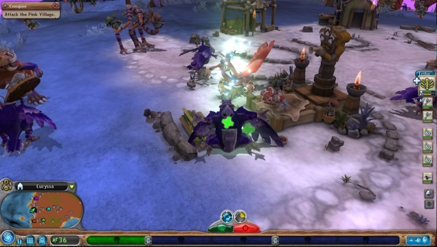
It probably doesn’t come as a huge surprise to note that I’m a nerd in all aspects of my life, not just my career. For me, this is particularly a love of video games. Rarely, however, do these two forms of nerdism coincide for me: while some games apply science and scientific theory, they are usually biased towards physics and engineering disciplines (looking at you, Portal). As far as my field is concerned, there are a few notable examples (such as Spore) which encapsulate the essence and majesty of evolution, but rarely do they incorporate the ‘genetic’ aspect that I love.
There’s nothing quite like making a horrific carnivorous monster and collapsing ecosystems by exterminating all of the wildlife, then taking over the Universe. Hmm…
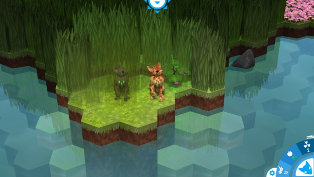
You can then imagine my utter delight at the discovery of a game that actually incorporates both population genetics and interesting gameplay. The indie survival game, aptly named Niche: A Genetics Survival Game, very literally represents this ‘niche’ for me (and I will not apologise for the pun!). Combining simplified models of population genetics processes such as genetic diversity, inbreeding (and associated inbreeding depression), natural selection, and stochastic events, Niche beautifully incorporates scientific theory (albeit toned down to a layman level) with challenging, yet engaging, gameplay mechanics and adorable art style.
Niche: A Genetics Survival Game epitomises the intersection of evolutionary theory and pop culture.
As one might expect from the title, Niche is at heart a survival game: the aim is to have your very own population of animals (dubbed ‘Nichelings’) survive the stresses of the world, through balancing population size, gene pools, resources (such as food, nests, space) and fighting off predators. Over time, the genetics component drives the evolution of your Nichelings, pushing them to be better at certain tasks depending on the traits selected for: the ultimate aim of the game is to create the perfectly adapted species that can colonise all of the land masses randomly generated.
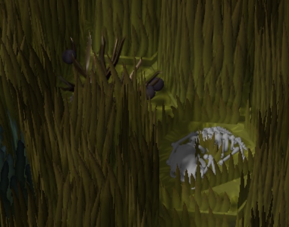
The user interface of Niche. A: The ranking of the selected Nicheling, moving from alpha, to beta, to gamma. This determines the order the Nichelings eat in (gammas get the short end of the stick). B: The traits of the selecting Nicheling. In order, these are the physical traits (i.e. the strength, speed and abilities of the animal), the genetic sequence (genotype) of the animal (expanded in C). the user-chosen mutations for that Nicheling and the pedigree of Nichelings. C: The expanded DNA sequence of the selected Nicheling, showing the paternal and maternal variants (alleles) of all the possible genes. Highlighted traits are the expressed trait (dominant) whilst the faded ones indicate recessive carrier genes that aren’t expressed. D: Collected food, one of the most important resources in the game. E: Nest material, required to build nests and produce offspring. F: The different senses (sight, smell, hearing) which can be toggled to give different viewpoints of the surrounding environments (with different benefits and weaknesses).
Niche requires cunning strategy, good foresight and planning, and sometimes a little luck. Although I’m decidedly not very good at Niche yet (I think my rates of extinction would mirror the real world a little too much for my liking…), the chance to involve my scientific background into my favourite hobby is a somewhat magical experience.
Oh god, I hope this isn’t a premonition for my career!
You might wonder why I care so much about a video game. While the game is in and of itself an interesting concept, to me it exemplifies one way we can make science an enjoyable and digestible concept for non-scientists. It’s possible that Niche could open the door of population-level genetics and evolution to a new audience, and potentially inspire the next generation of scientists in the field. Although that might be an extraordinarily long shot, it is my hope that the curiosity, mystery and creativity of scientific research is at least partially represented in media such as gaming to help integrate science and society.
Using video games for science?!
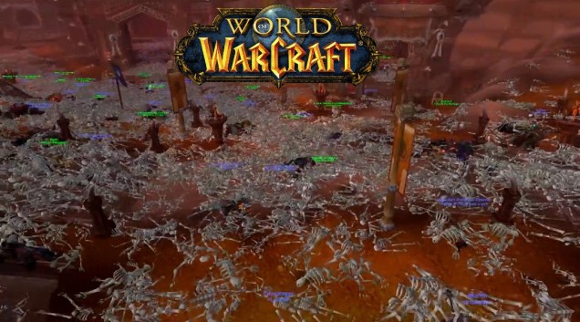
Both science and society can benefit from the (accurate) representation of science in pop culture, not just through fostering a connection between scientific theory and the recreational hobbies of people. In rare occasions, pop culture can even be used as a surrogate medium for testing scientific theories and hypotheses in a specific environment: for example, World of Warcraft has unwittingly contributed to scientific progress. As part of a particular boss battle, characters could become infected with a particular disease (called “Corrupted Blood”), which would have significant effects on players but only for a few seconds. While this was supposed to be removed after leaving the area of the fight, a bug in the game caused it to stay on animal pets that were afflicted, and thus become a viral phenomenon when it started to spread into the wider world (of Warcraft). The presence of the epidemic wiped out swathes of lower level players and caused significant social repercussions in the World of Warcraft community as players adjusted their behaviour to avoid or prevent transmission of the deadly disease.
This unique circumstance allowed a group of scientists to use it as a simulation of a real viral outbreak, as the spread of the disease was directly related to the social behaviour and interactivity of players within the game. The “Corrupted Blood” incident such enthralled scientists that multiplepapers were published discussing the feasibility of using virtual gaming worlds to simulate human reactions to epidemic outbreaks and viral transmissions on an unparalleled scale. Similarities between the method of transmission and behavioural responses to real-world events such as the avian flu epidemic were made.
And you thought Bird Flu was bad, at least they couldn’t teleport! Source: GameRant.
This isn’t the only example of even World of Warcraft informing research, with others using it to model economic theories through a free market auction system. While these may seem extraordinarily strange (to scientists and non-scientists alike), these examples demonstrate how popular media such as gaming can be an important interactive front between science and society.
Sometimes when I talk about the concept of conservation genetics to friends and family outside of the field, there can be some confusion about what this actually means. Usually, it’s assumed that means the conservation of genetics: that is, instead of trying to conserve individual animals or plants, we try to conserve specific genes. While in some cases this is partially true (there might be genes of particular interest that we want to maintain in a wild population), often what we actually mean is using genetic information to inform conservation management and to give us the best chance of long-term rescue for endangered species.
Don’t worry, it’s an open range zoo: the genes have plenty of room to roam.
See, the DNA of individuals contains much more information than just the genes that make up an organism. By looking at the number, frequency or distribution of changes and differences in DNA across individuals, populations or species, we can see a variety of different patterns. Typically, genetics-based conservation analysis is based on a single unifying concept: that different forces create different patterns in the genetic make-up of species and populations, and that these can be statistically evaluated using genetic data. The exact type or scale of effect depends on how the data is collected and what analysis we use to evaluate that data, although we could do multiple types of analysis using the same dataset.
Oftentimes, we want to know about the current or historical state of a species or population to best understand how to move forward: by understanding where a species has come from, what it has been affected by, and how it has responded to different pressures, we can start to suggest and best manage these species into the future.
However, there are lots of possible avenues for exploration: here are just a few…
Evolutionary significant units (ESUs) and management units (MUs)
One commonly used application of genetic information for conservation is the designation of what we call ‘Evolutionary Significant Units’ (ESUs). Using genetics, we can determine the boundaries of particular populations which correspond to their own unique evolutionary groups. These are often the results of historical processes which have separated and driven the independent evolution of each ESU, usually with low or no gene flow across these units. Generally, managing and conserving each of these can lead to overall more robust management of the species as a whole by making sure certain groups that have unique and potentially critical adaptations are maintained in the wild. Although ESUs can sometimes be arguable (particularly when there is some, but not much, gene flow across units), it forms an important aspect of conservation designations.
In cases of shorter term separations across these populations, where there are noticeable differences in the genetics of the populations but not necessarily massively different evolutionary histories, conservationists will sometimes refer to ‘Management Units’ (MUs). These have much weaker evolutionary pressure behind them but might be indicative of very recent impacts, such as human-driven fragmentation of habitat or contemporary climate change. MUs often reflect very sudden and recent changes in populations and might have profound implications for the future of these groups: thus, they are an important way of assessing the current state of the species. The next couple of figures demonstrate this from one of my colleagues’ research papers.
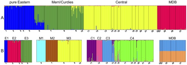
The geographic distributions of Yarra pygmy perch populations, generously taken from Brauer et al. (2013). Each dot and number on the map represents a single population of pygmy perch used in the analysis. The colour of the population represents which MU it belongs to, whilst the shape of the marker represents the ESU. To make this easier to visualise, the solid lines indicate the boundaries of ESUs while the dashed lines represent MU boundaries. You’ll notice that MUs are subsets of ESUs, and that Population 6 actually fits into two different ESUs: see below.An example of the output of an analysis (STRUCTURE) that determines population boundaries for Yarra pygmy perch using genetic data, generously taken from Brauer et al. (2013). Structure is an ‘assignment test’; using the input genetic information, it tries to make groups of individuals which are more similar to one another than other groups. In the graphs, each small column represents a single individual, with the colour bars representing how well it fits that (colour) population. The smaller numbers at the bottom and the labels above the graphs represent geographic populations (see the figure above).A) Shows the 4 major ESUs of Yarra pygmy perch, with some clear mixing between the Eastern ESU and the Merri/Curdies ESU in population 6. The rest of the populations fit pretty well entirely into one ESU. B) The MUs of Yarra pygmy perch, which shows the genetic structure within ESUs that can’t be seen well in A). Notice that some ESUs are made of many MUs (E.g. Central) while others are only one MU (e.g. MDB).
The two can be thought of as part of the same hierarchy, with ESUs reflecting more historic, evolutionary groups and MUs reflecting more recent (but not necessarily evolutionary) groups. For conservation management, this has traditionally meant that individuals from one ESU were managed independent of one another (to preserve their ‘pure’ evolutionary history) whilst translocations of individuals across MUs were common and often recommended. This is based on the idea that mixing very genetically different populations could cause adaptive genes in each population to become ‘diluted’, negatively affecting the ability of the populations to evolve: this is referred to as ‘outbreeding depression’ (OD).
Sometimes, adding something can make what you had even worse than before. The most depressing analogy of outbreeding depression; a ruined coffee.
However, more recent research has suggested that the concerns with OD from mixing across ESUs are less problematic than previously thought. Analysis of the effect of OD versus not supplementing populations with more genetic diversity has shown that OD is not the more dangerous option, and there is a current paradigm push to acknowledge the importance of mixing ESUs where needed.
Adaptive potential and future evolution
Understanding the genetic basis of evolution also forms an important research area for conservation management. This is particularly relevant for ‘adaptive potential’: that is, the ability for a particular species or population to be able to adapt to a variety of future stressors based on their current state. It is generally understood that having lots of different variants (alleles) of genes in the total population or species is a critical part of evolution: the more variants there are, the more choices there are for natural selection to act upon.
We can estimate this from the amount of genetic diversity within the population, as well as by trying to understand their previous experiences with adaptation and evolution. For example, it is predicted that species which occur in much more climatically variable habitats (such as in desert regions) are more likely to be able to handle and tolerate future climate change scenarios since they’ve demonstrated the ability to adapt to new, more extreme environments before. Examples of this include the Australian rainbowfishes, which are found in pretty well every climatic region across the continent (and therefore must be very good at adapting to new, varying habitats!).
Left: The distribution of rainbowfish across Australia, with each colour representing a particular ecotype. Right: A photo of a (very big) tropical rainbowfish taken from a recent MELFU field trip. Source: MELFU Facebook page. He really got around after that one stint in that children’s story.
Genetics-based breeding programs and pedigrees
A much more direct use of genetic information for conservation is in designing breeding programs. We know that breeding related individuals can have very bad results for offspring (this is referred to as ‘inbreeding depression’): so obviously, we would avoid breeding siblings together. However, in complex breeding systems (such as polygamous animals), or in wild populations, it can be very difficult to evaluate relationships and overall relatedness.
That’s where genetics comes in: by looking at how similar or different the DNA of two individuals are, we can not only check what relationship they are (e.g. siblings, cousins, or very distantly related) but also get an exact value of their genetic relatedness. Since we know that having a diverse gene pool is critical for future adaptation and survival of a species, genetics-based breeding programs can maximise the amount of genetic diversity in following generations. We can even use a computer algorithm to make the very best of breeding groups, using a quirky program called SWINGER.
If You Are the One, conservation genetics edition.
Taxonomy for conservation legislation
Another (slightly more complicated) application of genetics is the designation of species status. Large amounts of genetic information can often clarify complex issues of species descriptions (later issues of The G-CAT will discuss exactly how this works and why it’s not so straightforward…).
Why should we care what we call a species or not? Well, much of the protective legislation at the government level is designed at the species-level: legislative protections are often designated for a particular species, but doesn’t often distinguish particular populations. Thus, misidentified species can sometimes but lost if they were never detected as a unique species (and assumed to be just a population of another species). Alternatively, managing two species as one based on misidentification could mess with the evolutionary pathways of both by creating unfit hybrid species which do not naturally come into contact together (say, breeding individuals from one species with another because we thought they were the same species).
Awkward.
Additionally, if we assume that multiple different species are actually only one species, this can provide an overestimate of how well that species is doing. Although in total it might look like there are plenty of individuals of the species around, if this was actually made of 4 separate species then each one would be doing ¼ as well as we thought. This can feed back into endangered status classification and thus conservation management.
These are just some of the most common examples of applied genetics in conservation management. No doubt going into the future more innovative and creative methods of applying genetic information to maintaining threatened species and populations will become apparent. It’s an exciting time to be in the field and inspires hope that we may be able to save species before they disappear from the planet permanently.
Before we can delve too deep into the expansive world of molecular ecology (that is, the study of evolution using genetic information), we must first understand the basics of genetics.
All organisms (except some viruses, if you count those) contain DNA: you may have heard it referred to as ‘the building block of life’. And this is fundamentally true; DNA is a chemical compound contained within cells which acts as a technical blueprint the cell will use to make all of the parts of the body. In its stable state, DNA looks like a ‘twisted ladder’, or a ‘double helix’ as we call it. The rungs of the DNA ladder are made of a combination of ‘nucleotide bases’, which are shortened to G (guanine), C (cytosine), A (adenosine) and T (thymine). Hopefully, these letters look a little familiar (see the top of the page…). Each one of these is always paired with a specific base: A is always paired with T, G with C. One ‘pair’ of sequences makes up one rung of the ladder.
The (very simplified) structure of the DNA double helix. Bonus points if you spot the blog title.
These letters of the DNA more-or-less spell out the basis for making all of the different proteins of the body. Specific sequences will say, for example, where to start reading the code (the capital at the start of the sentence) for a particular protein, while others will tell it where to stop (the full stop at the end of the sentence). The rest of the sentence is translated into the protein and is what we call a ‘gene’.
Despite the importance of genes, not all of the DNA is actually made of them. In fact, it’s estimated that only 1.5% of the genome (that is, the collection of all the DNA sequence in an organism) consists of genes: the rest of it is attributed to other things like control sequences, ‘junk’ DNA or coding for non-proteins (like RNAs, another type of nucleic acid). Some sections of the DNA sequence are often ‘cut out’ during the process of translating the gene into a protein; these are call ‘introns’ and are considered non-coding regions. It’s sort of like when you’re 100 words over the word count of an essay and have to start chopping sentences into smaller pieces. The parts that aren’t cut out, and actually translate to the protein, are called ‘exons’.
While the exact code of the gene is important, not all genes are expressed at the same time or constantly. Many genes are ‘switched on’ (activated) or ‘switched off’ (deactivated) by other external influences; usually different micro-sequences or proteins which block off or allow the translation process to occur. For example, the gene that creates the protein to digest lactose isn’t always active: only when lactose enters the cell and binds to a specific protein that rests on top of the lactose-digesting gene, removing it, does translation start to happen. This is because it’d be a total waste to make lactose-digesting proteins if there was no lactose around at all.
The generalised structure of the genome. Note that much of it is not made of genes. Within the gene, only the exon regions are translated into the final protein; the intron sequences are removed in an intermediate copy of the DNA (call the ‘mRNA’). The expression of the gene is controlled by the presence or absence of the repressor protein.
Why does all of this matter for molecular ecology? Well, the DNA sequence changes over generations due to mutations (spoiler: they don’t usually turn your skin green); these can happen for a variety of different reasons and aren’t inherently good or bad. It really depends where these mutations are happening in the genome and how this changes the DNA and the downstream proteins (or not).
Thus, DNA evolves over time if new mutations arise which cause changes that natural selection favours: if a mutation makes an animal see better at night, then it might gradually evolve to become a night hunter as it accumulates new mutations (if there is an actual fitness benefit to doing so: we’ll discuss that more in a later post). Contrastingly, bad mutations which cause an organism to be very “maladaptive” (i.e. “bad”; say, mutations which make your eyes bleed constantly) would be selected against.
We can use these types of information to study the evolution, ecology and conservation status of a species or population. We can look at how these mutations have accumulated; where in the genome they have accumulated; how frequently these new mutations arise; what effect these mutations have on the organism. With different statistical models, we can start to build a quantifiable way to handle this data and voila: molecular ecology is born! Many of these models are based on mathematical correlations between certain patterns in the frequency and distribution of new mutations within populations or species and certain biological effects like the size of the population, natural selection or connectivity across populations. Thus, we can investigate a massive swathe of possible questions with genetic data!