In one form or another, you may have been (unfortunately) exposed to the notion of ‘testing for someone’s race using genetics.’ In one sense, this is part of the motivation and platform of ‘23andMe’, which maps the genetic variants across the human genome back to likely origin populations to determine the relative ancestry of a person. In a much darker sense, the connection between genetic identity and race is the basis of eugenics, by suggesting genetic “purity” (this concept is utter nonsense, for reference) of a population as justification for some racist hierarchy. Typically, this is associated with Hitler’s Nazism, but more subversive versions of this association still exist in the world: for Australian readers, most notably when the far-right conservative minor party One Nation suggested that people claiming to be Indigenous should be subjected to genetic testing to verify their race.
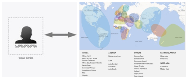
A simplified overview of how DNA Ancestry methods work, by associating particular genetic variants within your genome to likely regions of origin. Note the geographic imprecision in the method on the map on the right, as well as the clear gaps. Source: Ancestry blog.
The biological concept of a ‘race’
Beyond the apparent ethical and moral objections to the invasive nature of demanding genetic testing for Indigenous peoples, a crucial question is one of feasibility: even if you decided to genetically test for race, is this possible? It might come as a surprise to non-geneticists that actually, from a genetic perspective, race is not a particularly stable concept.
James Watson himself. I bet Rosalind Franklin never said anything like this… Source: Wikipedia.
You might ask: why is that? There are perceivable differences in the various peoples of the world, surely some of those could be related to both a ‘race’ and a ‘genetic identity’, right? Well, the issue is primarily due to the lack of identifiability of genetic variants that can be associated with a race. Decades of research in genetic variation across the global human population indicates that, due to the massive size of the human population and levels of genetic variation, it is functionally impossible to pinpoint down genetic variants that uniquely identify a ‘race’. Human genetic variation is such a beautiful spectrum of alleles that it becomes impossible to reliably determine where one end of the spectrum ends or begins, or to identify a strict number of ‘races’ within the kaleidoscope of the human genome.
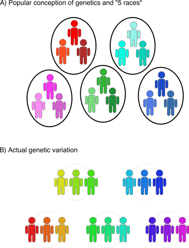
A diagram of exactly why identifying a genetic basis for race is impossible in humans. A) The ‘idealised’ version of race; people are easily classified by their genetic identity, with some variation within each classification (in this case, race) but still distinctiveness between them. B) The reality of human genetic variation, which makes it exceedingly difficult to make any robust or solid boundaries between groups of people due to the sheer amount of variation. Source: Harvard University blog.
This is exponentially difficult for people who might have fewer sequenced ancestors or relatives; without the reference for genetic variation, it can be even harder to trace their genetic ancestry. Such is the case for Indigenous Australians, for which there is a distinct lack of available genetic data (especially compared to European-descended Australians).
The non-genetic components
The genetic non-identifiability of race is but one aspect which contradicts the rationality of genetic race testing. As we discussed in the previous post on The G-CAT, the connection between genetic underpinning and physicality is not always clear or linear. The role of the environment on both the expression of genetic variation, as well as the general influence of environment on aspects such as behaviour, philosophy, and culture necessitate that more than the genome contributes to a person’s identity. For any given person, how they express and identify themselves is often more strongly associated with their non-genetic traits such as beliefs and culture.
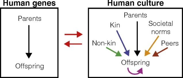
A comparison of genetic vs. cultural inheritance, which demonstrates (as an example) how other factors (in this case, other people) influence the passing on of cultural traits. Remember that this but one aspect of the factors that determine culture and identity, and equally (probably more) complex networks exist for other influences such as environment and development. Source: Creanza et al. (2017), PNAS.
These factors cannot reliably be tested under a genetic framework. While there may be some influence of genes on how a person’s psychology develops, it is unlikely to be able to predict the lifestyle, culture and complete identity of said person. For Indigenous Australians, this has been confounded by the corruption and disruption of their identity through the Stolen Generation. As a result, many Indigenous descendants may not appear (from a genetic point of view) to be purely Indigenous but their identity and culture as an Indigenous person is valid. To suggest that their genetic ancestry more strongly determines their identity than anything else is not only naïve from a scientific perspective, but nothing short of a horrific simplification and degradation of those seeking to reclaim their identity and culture.
The non-identifiability of genetic race
The science of genetics overwhelmingly suggests that there is no fundamental genetic underpinning of ‘race’ that can be reliably used. Furthermore, the impact of non-genetic factors on determining the more important aspects of personal identity, such as culture, tradition and beliefs, demonstrates that attempts to delineate people into subcategories by genetic identity is an unreliable method. Instead, genetic research and biological history fully acknowledges and embraces the diversity of the global human population. As it stands, the phrase ‘human race’ might be the most biologically-sound classification of people: we are all the same.
Note: For some clear, interesting presentations on the topic of de-extinction, and where some of the information for this post comes from, check out this list of TED talks.
The current conservation crisis
The stark reality of conservation in the modern era epitomises the crisis disciplinethat so often is used to describe it: species are disappearing at an unprecedented rate, and despite our best efforts it appears that they will continue to do so. The magnitude and complexity of our impacts on the environment effectively decimates entire ecosystems (and indeed, the entire biosphere). It is thus our responsibility as ‘custodians of the planet’ (although if I had a choice, I would have sacked us as CEOs of this whole business) to attempt to prevent further extinction of our planet’s biodiversity.
At least from a genetic perspective, this sometimes involves trying to understand the nature and potential of adaptation from genetic variation (as a predictor of future adaptability). Or using genetic information to inform captive breeding programs, to allow us to boost population numbers with minimal risk of inbreeding depression. Or perhaps allowing us to describe new, unidentified species which require their own set of targeted management recommendations and political legislation.
How my overactive imagination pictures ‘genetic rescue’.
There’s one catch (well, a few really) with genetic rescue: namely, that one must have other populations to ‘outbreed’ with in order add genetic variation to the captive population. But what happens if we’re too late? What if there are no other populations to supplement with, or those other populations are also too genetically depauperate to use for genetic rescue?
Believe it or not, sometimes it’s not too late to save species, even after they have gone extinct. Which brings us from this (lengthy) introduction to this week’s topic: de-extinction. Yes, we’re literally (okay, maybe not) going to raise the dead.
Your textbook guide to de-extinction. Now banned in 47 countries.
Backbreeding: resurrection by hybridisation
You might wonder how (or even if!) this is possible. And to be frank, it’s extraordinarily difficult. However, it has to a degree been done before, in very specific circumstances. One scenario is based on breeding out a species back into existence: sometimes we refer to this as ‘backbreeding’.
This practice really only applies in a few select scenarios. One requirement for backbreeding to be possible is that hybridisation across species has to have occurred in the past, and generally to a substantial scale. This is important as it allows the genetic variation which defines one of those species to live on within the genome of its sister species even when the original ‘host’ species goes extinct. That might make absolutely zero sense as it stands, so let’s dive into this with a case study.
A map of the Galápagos archipelago and tortoise species, with extinct species indicated by symbology. Lonesome George was the last known living member of the Pinta Island tortoise, C. abingdonii for reference. Source: Wikipedia.
One of these species, Chelonoidis elephantopus, also known as the Floreana tortoise after their home island, went extinct over 150years ago, likely due to hunting and trade. However, before they all died, some individuals were transported to another island (ironically, likely by mariners) and did the dirty with another species of tortoise: C. becki. Because of this, some of the genetic material of the extinct Floreana tortoiseintrogressed into the genome of the still-living C. becki. In an effort to restore an iconic species, scientists from a number of institutions attempted to do what sounds like science-fiction: breed the extinct tortoise back to life.
When you saw the title for this post, you were probably expecting some Jurassic Parklevel ‘dinosaurs walking on Earth again’ information. I know I did when I first heard the term de-extinction. Unfortunately, contemporary de-extinction practices are not that far advanced just yet, although there have been some solid attempts. Experiments conducted using the genomic DNA from the nucleus of a dead animal, and cloning it within the egg of another living member of that species has effectively cloned an animal back from the dead. This method, however, is currently limited to animals that have died recently, as the DNA degrades beyond use over time.
The same methods have been attempted for some extinct animals, which went extinct relatively recently. Experiments involving the Pyrenean ibex (bucardo) were successful in generating an embryo, but not sustaining a living organism. The bucardo died 10 minutes after birth due to a critical lung condition, as an example.
The challenges and ethics of de-extinction
One might expect that as genomic technologies improve, particularly methods facilitated by the genome-editing allowed from CRISPR/Cas-9 development, that we might one day be able to truly resurrect an extinct species. But this leads to very strongly debated topics of ethics and morality of de-extinction. If we can bring a species back from the dead, should we? What are the unexpected impacts of its revival? How will we prevent history from repeating itself, and the species simply going back extinct? In a rapidly changing world, how can we account for the differences in environment between when the species was alive and now?
The Chaotic Neutral (?) approach to de-extinction.
There is no clear, simple answer to many of these questions. We are only scratching the surface of the possibility of de-extinction, and I expect that this debate will only accelerate with the research. One thing remains eternally true, though: it is still the distinct responsibility of humanity to prevent more extinctions in the future. Handling the growing climate change problem and the collapse of ecosystems remains a top priority for conservation science, and without a solution there will be no stable planet on which to de-extinct species.
You bet we’re gonna make a meme months after it’s gone out of popularity.
A number of timesbefore on The G-CAT, we’ve discussed the idea of using the frequency of different genetic variants (alleles) within a particular population or species to test a number of different questions about evolution, ecology and conservation. These are all based on the central notion that certain forces of nature will alter the distribution and frequency of alleles within and across populations, and that these patterns are somewhat predictable in how they change.
One particular distinction we need to make early here is the difference between allele frequency and allele identity. In these analyses, often we are working with the same alleles (i.e. particular variants) across our populations, it’s just that each of these populations may possess these particular alleles in different frequencies. For example, one population may have an allele (let’s call it Allele A) very rarely – maybe only 10% of individuals in that population possess it – but in another population it’s very common and perhaps 80% of individuals have it. This is a different level of differentiation than comparing how different alleles mutate (as in the coalescent) or how these mutations accumulate over time (like in many phylogenetic-based analyses).
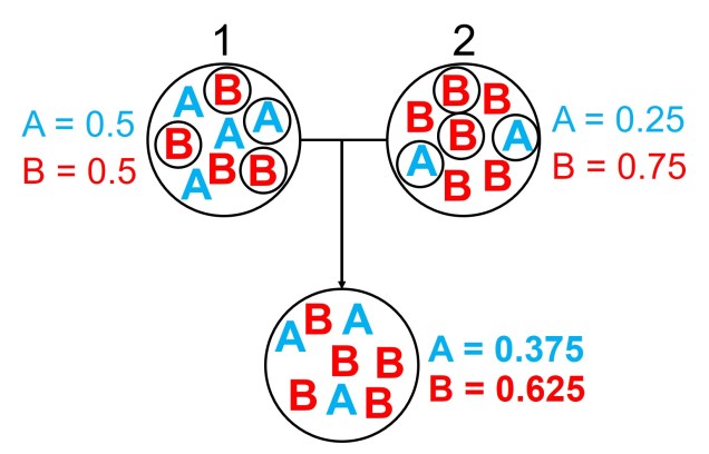
An example of the difference between allele frequency and identity.In this example (and many of the figures that follow in this post), the circle denote different populations, within which there are individuals which possess either an A gene (blue) or a B gene. Left: If we compared Populations 1 and 2, we can see that they both have A and B alleles. However, these alleles vary in their frequency within each population, with an equal balance of A and B in Pop 1 and a much higher frequency of B in Pop 2. Right: However, when we compared Pop 3 and 4, we can see that not only do they vary in frequencies, they vary in the presence of alleles, with one allele in each population but not the other.
An example of how gene flow across populations homogenises allele frequencies. We start with two initial populations (1 and 2 from above), which have very different allele frequencies. Hybridising individuals across the two populations means some alleles move from Pop 1 and Pop 2 into the hybrid population: which alleles moves is random (the smaller circles). Because of this, the resultant hybrid population has an allele frequency somewhere in between the two source populations: think of like mixing red and blue cordial and getting a purple drink.
An example of a Structure plot which long-term The G-CAT readers may be familiar with. This is taken from Brauer et al. (2013), where the authors studied the population structure of the Yarra pygmy perch. Each small column represents a single individual, with the colours representing how well the alleles of that individual fit a particular genetic population (each population has one colour). The numbers and broader columns refer to different ‘localities’ (different from populations) where individuals were sourced. This shows clear strong population structure across the 4 main groups, except for in Locality 6 where there is a mixture of Eastern and Merri/Curdies alleles.
Determining genetic bottlenecks and demographic change
A diagram of how allele frequencies change in genetic bottlenecks due to genetic drift. Left: Large circles again denote a population (although across different sequential times), with smaller circle denoting which alleles survive into the next generation (indicated by the coloured arrows). We start with an initial ‘large’ population of 8, which is reduced down to 4 and 2 in respective future times. Each time the population contracts, only a select number of alleles (or individuals) ‘survive’: assuming no natural selection is in process, this is totally random from the available gene pool. Right: We can see that over time, the frequencies of alleles A and B shift dramatically, leading to the ‘extinction’ of Allele B due to genetic drift. This is because it is the less frequent allele of the two, and in the smaller population size has much less chance of randomly ‘surviving’ the purge of the genetic bottleneck.
An example of how the frequency of alleles might vary under natural selection in correlation to the environment. In this example, the blue allele A is adaptive and under positive selection in the more intense environment, and thus increases in frequency at higher values. Contrastingly, the red allele B is maladaptive in these environments and decreases in frequency. For comparison, the black allele shows how the frequency of a neutral (non-adaptive or maladaptive) allele doesn’t vary with the environment, as it plays no role in natural selection.
Fixed differences are sometimes used as a type of diagnostic trait for species. This means that each ‘species’ has genetic variants that are not shared at all with its closest relative species, and that these variants are so strongly under selection that there is no diversity at those loci. Often, fixed differences are considered a level above populations that differ by allelic frequency only as these alleles are considered ‘diagnostic’ for each species.
An example of the difference between fixed differences and allelic frequency differences. In this example, we have 5 cats from 3 different species, sequencing a particular target gene. Within this gene, there are three possible alleles: T, A or G respectively. You’ll quickly notice that the T allele is both unique to Species A and is present in all cats of that species (i.e. is fixed). This is a fixed difference between Species A and the other two. Alleles A and G, however, are present in both Species B and C, and thus are not fixed differences even if they have different frequencies.
To distinguish between the two, we often use the overall frequency of alleles in a population as a basis for determining how likely two individuals share an allele by random chance. If alleles which are relatively rare in the overall population are shared by two individuals, we expect that this similarity is due to family structure rather than population history. By factoring this into our relatedness estimates we can get a more accurate overview of how likely two individuals are to be related using genetic information.
The wild world of allele frequency
Despite appearances, this is just a brief foray into the many applications of allele frequency data in evolution, ecology and conservation studies. There are a plethora of different programs and methods that can utilise this information to address a variety of scientific questions and refine our investigations.
Since evolution is a constant process, occurring over both temporal and spatial scales, the impact of evolutionary history for current and future species cannot be overstated. The various forces of evolution through natural selection have strong, lasting impacts on the evolution of organisms, which is exemplified within the genetic make-up of all species. Phylogeography is the domain of research which intrinsically links this genetic information to historical selective environment (and changes) to understand historic distributions, evolutionary history, and even identify biodiversity hotspots.
The Ice Age(s)
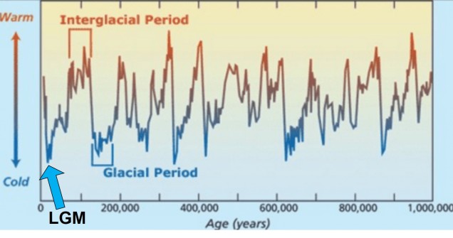
Although there are a huge number of both historic and contemporary climatic factors that have influenced the evolution of species, one particularly important time period is referred to as the Pleistocene glacial cycles. The Pleistocene epoch spans from ~2 million years ago until ~100,000 years ago, and is a time of significant changes in the evolution of many species still around today (particularly for vertebrates). This is because the Pleistocene largely consisted of several successive glacial periods: at times, the climate was significantly cooler, glaciers were more widespread and sea-levels were lower (due to the deeper freezing of water around the poles). These periods were then followed by ‘interglacial periods’, where much of the globe warmed, ice caps melted and sea-levels rose. Sometimes, this natural pattern is argued as explaining 100% of recent climate change: don’t be fooled, however, as Pleistocene cycles were never as dramatic or irreversible as modern, anthropogenically-driven climate change.
The general pattern of glacial and interglacial periods over the last 1 million years, adapted from Oceanbites.
The glacial cycles of the Pleistocene had a number of impacts on a plethora of species on Earth. For many of these species, these glacial-interglacial periods resulted in what we call ‘glacial refugia’ and ‘interglacial expansion’: at the peak of glacial periods, many species’ distributions contracted to small patches of suitable habitat, like tiny islands in a freezing ocean. As the globe warmed during interglacial periods, these habitats started to spread and with them the inhabiting species. While it’s expected that this likely happened many times throughout the Pleistocene, the most clearly observed cycle would be the most recent one: referred to as the Last Glacial Maximum (LGM), at ~21,000 years ago. Thus, a quick dive into the literature shows that it is rife with phylogeographic examples of expansions and contractions related to the LGM.
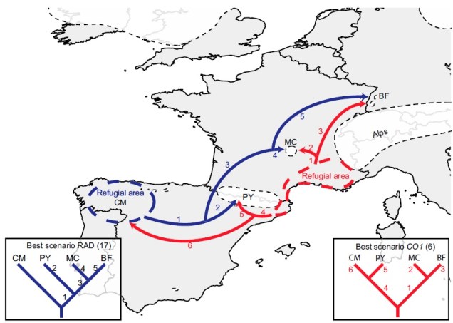
An example of how phylogeographic analysis can find glacial refugia in species, in this case the montane caddisfly Thremma gallicum from Macher et al. (2017). The colours refer to the two datasets they used (blue = ddRADseq; red = mtDNA) and the arrows demonstrate migration pathways in the interglacial period following the LGM.
And this loss of genetic diversity isn’t just a hypothetical, or an interesting note in evolution. It can have dire impacts for the survivability of species. Take for example, the very charismatic cheetah. Like many large, apex predator species, the cheetah in the modern day is endangered and at risk of extinction to a variety of threats, and although many of these are linked to modern activity (such as being killed to protect farms or habitat clearing), some of these go back much further in history.
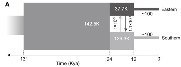
Believe it not, the cheetah as a species actually originated from an ancestor in the Americas: they’re closely related to other American big cats such as the puma/cougar. During the Miocene (5 – 8 million years ago), however, the ancestor of the modern cheetah migrated a very long way to Africa, diverging from its shared ancestor with jaguarandi and cougars. Subsequent migrations into Africa and Asia (where only the Iranian subspecies remains) during the Pleistocene, dated at ~100,000 and ~12,000 years ago, have been shown through whole genome analysis to have resulted in significant reductions in the genetic diversity of the cheetah. This timing correlates with the extinction of the cheetah and puma within North America, and the worldwide extinction of many large mammals including mammoths, dire wolves and sabre-tooth tigers.
The demographic history of the African cheetah population, based on whole genomes in Dobrynin et al. (2015). In this figure, ‘Eastern’ refers to a Tanzanian population whilst ‘southern’ refers to a Namibian population (and as such doesn’t depict bottlenecks elsewhere in the cheetah e.g. Iran). The initial population underwent a severe genetic bottleneck ~12,000 years ago, likely due to glaciation.
Examples of the incredibly low genetic diversity in cheetah, both from Dobrynin et al. (2015). A) shows the relative level of genetic diversity in cheetah compared to many other species, being lower than Tasmanian Devils and significantly lower than humans and domestic cats. D) shows the overall variation across the genome of a domestic cat (top), the inbred Abyssinian cat (middle) and the cheetah (bottom). Highly variable regions are indicated in red, whilst low variability regions are indicated in green. As you can see, the entirety of the cheetah genome has incredibly low genetic variation, even compared to another cat species considered to have low genetic variation (the Abyssinian).
Inference for the future
Understanding the impact of the historic environment on the evolution and genetic diversity of living species is not just important for understanding how species became what they are today. It also helps us understand how species might change in the future, by providing the natural experimental evidence of evolution in a changing climate.