The G-cat

The utility of a reference genome

In the 18 years since the completion of the Human Genome Project, the practicality of assembling full genomes for a wide range of taxa beyond ourselves has only improved. While model taxa systems have achieved genomes before many others, it is now possible for whole genomes to be assembled for a range of non-model organisms as well. But how do we assemble the genome of a species for the very first time (often de novo – literally “from the new”)? What can we do with this genome? Why is it so useful? Let’s delve into the process and outcomes of genome assembly a little more.

How to assemble a genome

While there are a number of steps to the genome assembly process, it’s not overly different (at least in terms of the initial work) to what we do for reduced-representation sequencing methods such as ddRAD-seq (more on that here). Essentially, we need to extract high-quality DNA from a tissue sample of one individual, thoroughly sequence this DNA, and then assemble the fragments (‘reads’) of this sequencing into a contiguous set of nucleotides (or as best as possible). Of course, the bioinformatic component of this pipeline is the trickiest, and there are a number of crucial considerations that need to be made throughout the process (some of which differ from the other non-whole-genome methods).

Extracting the DNA

As with all sequencing methods, the first step in the process is to extract DNA from a tissue sample. For example, in our fish work we generally extract this DNA from small clippings from the anal fin (which doesn’t harm the fish or affect their overall swimming capacity), or from muscle tissue samples (e.g., if we’re working with museum samples). The quantity and purity of DNA required is often much higher for whole genome assemblies compared to our other genomic methods – we want to make sure we have really good coverage (more on that in a minute) of the entire genome of a single (or a few) individual(s). One other aspect that might be different is that it’s actually easier to assemble the genome of an inbred individual compared to one hosting lots of genetic diversity. Variations between the two sets of chromosomes in a single individual can impact on how easy it is to assemble fragments in the later bioinformatic stages (or to distinguish from sequencing errors). That’s not to say you can’t sequence the genome of a diverse individuals, but it might be adding a bit of a headache later.

Another thing that needs to be considered is the size of the genome in question: within teleost fish alone, genomes can be anywhere between 400 million (smooth pufferfish) and 43 billion (Australian lungfish) base pairs long (for reference, the human genome is around 3.1 billion base pairs long). As you can imagine, the bigger the genome the more DNA you’ll need to adequately cover it with reasonable accuracy. Similarly, the number of copies of each chromosome an organism possesses (‘ploidy’) creates additional problems both at the pre- and post-sequencing steps – more on that later.

Assembling the genome

Once we’ve obtained our mountain of genomic sequences, we set upon the gargantuan task of bioinformatic analysis. There are a lot of different considerations and challenges to tackle when handling such a massive amount of data – let’s go through some of them here.

Coverage

One of the most relevant factors in creating an effective genome is based upon what we call coverage. This can mean a few different things based on context, so I’ll specify coverage breadth and depth here. Coverage breadth is the total length of your target genome that is covered by your sequences – ideally, this should of course by 100%, but some parts of the genome are particularly challenging to sequence (e.g. repetitive regions, or those with high GC content) and might be missing from your data. On top of that is coverage depth, which is the number of times a particular region has been sequenced in one of our fragments. Good depth is important to ensure accuracy – since sequencing machines occasionally make errors, high coverage can help us identify the true nucleotide at a given base pair (as well as distinguishing between errors and heterozygous sites).

Ploidy

For some organisms, the number of copies of a chromosome (ploidy) it possesses may also bring another challenge. In general, despite the ploidy of an organism reference genomes are usually only a haploid sequence, with a single representative genome. For humans, we’re blessed with only two copies of the genome (diploid), which means with good enough coverage we can separate the two to obtain our haploid sequence. Some species, though – like salmonids and some plants – can have much higher ploidy, such as hexaploidy. Not only does this mean we have to work with six copies of the same genome, but each one of these copies might have wildly different gene functions and evolutionary histories. This can cause absolute chaos, and I do not envy anyone who has to deal with them!

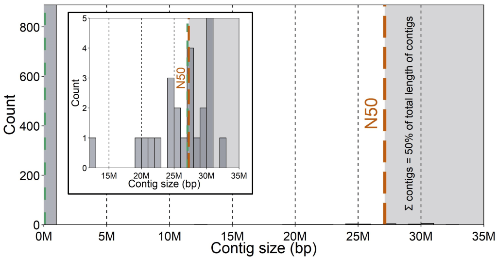
N50

One of the most commonly used measures of genome assembly quality is called the N50 statistic. The N50 of an assembly is the length of the smallest contig above which the combined contigs contain 50% of the total length of all contigs combined. That is, all of the contigs bigger than the N50 should combine to constitute 50% of all contigs in length. Because there can be a lot of variation in the length of contigs (often many very short ones and few very large ones), the N50 helps capture the relative abundance of big (“good”) contigs in the assembly. Other valuable statistics to report are the number of contigs in total and their average length, as well as the average sequencing depth across the genome.

Chromosomes

If the genome assembly is particularly great, contiguous sequences might be able to be built into chromosomes. This usually requires using a related species’ genome as an anchor in order to assign contigs to chromosomes – this process can also help to identify gaps in the genome where the relevant contig is missing (assuming, of course, that the reference used is not massively genetically divergent from your target genome assembly species).

Annotating the genome

Once we have an assembled genome, the next step is usually to generate an annotated one. This means that (beyond just having the full DNA sequence of an organism’s genome) we can delineate where the genes are, what their functions or roles are, as well as other components of the genome such as repeat or non-coding regions. The first major step of annotation involves predicting the location and sequence of genes within the genome by using information from various databases. If similar species already possess an annotated genome, we might be able to simply delineate genes based on the similarity of our genome sequence to the identified genes in the reference species. Similarly, we can reverse-engineer the gene sequence from the expressed RNA (transcripts) or protein sequences to determine the underlying genomic sequence and thus gene location. While references from more similar species are more likely to match the genome of our target species (and also have similar biological function), some broad databases (e.g. from all fish) can still be useful for particularly conserved genes. Additionally, if we have transcript data from our own species (even the same individual), we can similarly delineate the genes responsible by converting the transcript sequence to the underlying genomic code. Once we have managed to predict and delineate our genes, the next major step is to assign a biological function to these genes – also through data repositories (although this information can also come from more targeted, gene-specific information such as from medical research).

Linkage maps

Another useful extension for an assembled genome is the estimation of a ‘linkage map’ – this effectively determines regions (or their overall size) in the genome which are likely to be co-inherited, either because of their physical proximity or due to inter-region interactions. Particularly, linkage maps are useful to determine how widely selection on a single locus may impact neighbouring sequences, which is an important factor in detecting regions under selection or determining evolutionary histories.

Linkage maps are a little harder to determine – you need to not only know the physical location of alleles across the genome, but also estimate how likely different loci are likely they are to be jointly inherited in future offspring. To do this, we have to obtain the whole genome of not only at least one reference individual, but the whole genomes of several offspring in a pedigree-like analysis. This way, we can look at how various sections of the genome (‘blocks’) are inherited from either the maternal or paternal parent in their offspring – in general, we might expect that blocks are larger in populations with lower genome-wide diversity and in regions where natural selection might act against recombination. The more parent and offspring combinations, the better we can estimate these linkage blocks across the genome. These linkage blocks can tell us a lot about both adaptive and neutral (i.e. demographic) evolution in species over time, and are an important component of many whole-genome studies.

Conclusions

Assembling and annotating a brand new reference genome certainly has it’s bioinformatic challenges – many of which were not touched on in great detail here. However, they remain an extremely useful resource for studying the evolution, conservation and management of a wide range of species, and are become readily more available to non-model species as time progresses. Maybe one day, we will have achieved the ultimate goal of sequencing the genome of every species on the planet – until then, we’ll keep on assembling!